

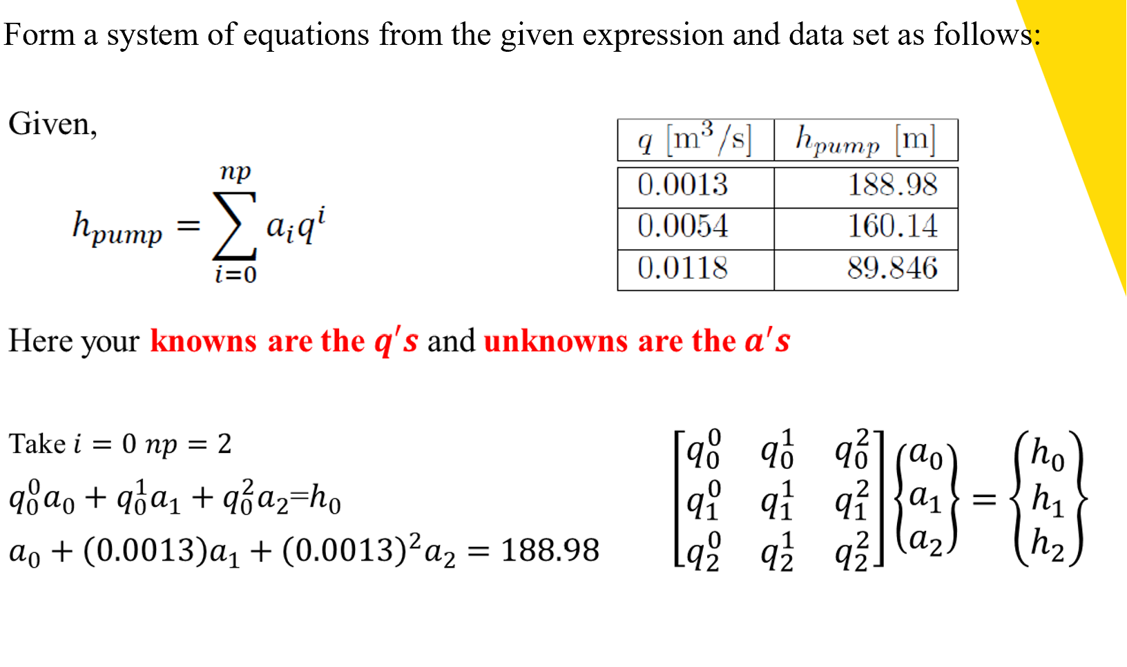
Question: Form a system of equations from the given expression and data set as follows: Given, np hpump = [aq i=0 q [m/s] hpump [m]
![as follows: Given, np hpump = [aq i=0 q [m/s] hpump [m]](https://dsd5zvtm8ll6.cloudfront.net/si.experts.images/questions/2024/02/65cb73cea4867_27065cb73ce7d251.jpg)
![a's 0 9 91 0 91 9 q1 92 9/2 9] (ao](https://dsd5zvtm8ll6.cloudfront.net/si.experts.images/questions/2024/02/65cb73d02e2b8_27265cb73d004f89.jpg)
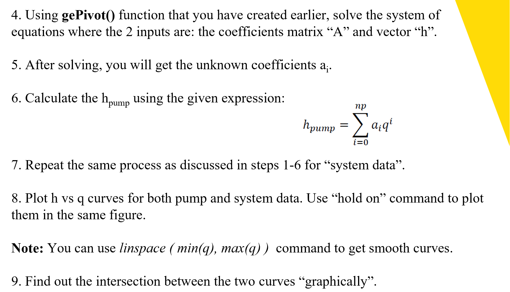
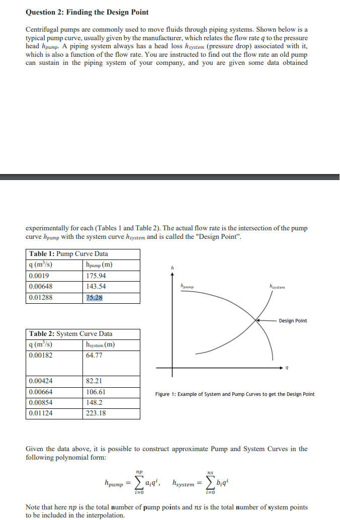
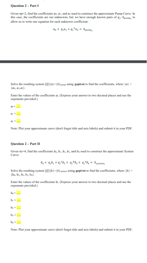
Form a system of equations from the given expression and data set as follows: Given, np hpump = [aq i=0 q [m/s] hpump [m] 188.98 160.14 89.846 Take i = 0 np = 2 qao + qa + qa=ho ao + (0.0013) a + (0.0013)a = 188.98 0.0013 0.0054 0.0118 Here your knowns are the q's and unknowns are the a's 0 9 91 0 91 9 q1 92 9/2 9] (ao q 9a}= (a) 2 q 9. 2 ho h h 2. Create "q" array and h column vector from the given data. 3. This structure is known as a Vandermonde matrix, and can easily be generated with the right commands in MATLAB. Create a vector q [q0 q1 q2] Create the Vandermonde matrix V = vander (q) Flip left/right (default convention in MATLAB Q fliplr (V) or Q fliplr (vander (q)) = = = 0 [98 0 qi 2 996 2 q1 q 0 2 92 9 9 4. Using gePivot() function that you have created earlier, solve the system of equations where the 2 inputs are: the coefficients matrix "A" and vector h. 5. After solving, you will get the unknown coefficients a. 6. Calculate the hpump using the given expression: np hpump = aq i=0 7. Repeat the same process as discussed in steps 1-6 for "system data. 8. Plot h vs q curves for both pump and system data. Use "hold on" command to plot them in the same figure. Note: You can use linspace (min(q), max(q)) command to get smooth curves. 9. Find out the intersection between the two curves "graphically". Question 2: Finding the Design Point Centrifugal pumps are commonly used to move fluids through piping systems. Shown below is a typical pump curve, usually given by the manufacturer, which relates the flow rate q to the pressure head hpump. A piping system always has a head loss hsystem (pressure drop) associated with it, which is also a function of the flow rate. You are instructed to find out the flow rate an old pump can sustain in the piping system of your company, and you are given some data obtained experimentally for each (Tables 1 and Table 2). The actual flow rate is the intersection of the pump curve hpump with the system curve hsystem and is called the "Design Point". Table 1: Pump Curve Data q (m/s) 0.0019 0.00648 0.01288 hpump (m) 175.94 143.54 75.28 Table 2: System Curve Data q (m/s) hsystem (m) 0.00182 64.77 0.00424 0.00664 0.00854 0.01124 82.21 106.61 148.2 223.18 hpump np hpump = [9;9, hsystem = i=0 heystem Figure 1: Example of System and Pump Curves to get the Design Point i=0 Design Point Given the data above, it is possible to construct approximate Pump and System Curves in the following polynomial form: biq 9 Note that here np is the total number of pump points and ns is the total number of system points to be included in the interpolation. Question 2 - Part I Given np-2, find the coefficients ao, ai, and az used to construct the approximate Pump Curve. In this case, the coefficients are our unknowns, but we have enough known pairs of qj, hpump, to allow us to write one equation for each unknown coefficient: ao+qja + aa=hpump, Solve the resulting system [Q]{a}={hpump using gepivot to find the coefficients, where {a} = {ai, ai,az). Enter the values of the coefficients al. (Express your answer to two decimal places and use the exponents provided.) al Note: Plot your approximate curve (don't forget title and axis labels) and submit it in your PDF. Question 2 - Part II Given ns-4, find the coefficients bo, bi, b2, b3, and b4 used to construct the approximate System Curve: bo+qb+q,b + q,b+ qjb = hsystem/ Solve the resulting system [Q] {b}={k} system using gepivot to find the coefficients, where {b} = {bo, bi, bz, bs, b4). Enter the values of the coefficients b. (Express your answer to two decimal places and use the exponents provided.) bo= b = b = b3 = b4 =.... Note: Plot your approximate curve (don't forget title and axis labels) and submit it in your PDF. Question 2 - Part III Calculate the Design Point (DP) i.e. the values of q and h at the intersection of the pump and system curves. Use the np-2 Pump Curve and the ns-4 System Curve. Plot your approximate pump and system curves together on one figure to visualize the design point and submit the plot in your PDF. Don't forget title, axis labels, and legend. Enter the design point (DP). (Express your answer to three significant digits for q and to two decimal places for h) q=.... (m/s) h =.... (m) Note: Begin by identifying what type of problem this is. Question 2 - Part IV Find two alternative approximations to the design point. 1. The first obtained with ns-2, using the first three system data points. Plot your approximate pump and system curves (ns-2) together on one figure to visualize the design point and submit the plot in your PDF. Don't forget title, axis labels, and legend. Enter the values of the coefficients be using the first three system data points. (Express your answers to two decimal places and use the exponents provided). bo= .... b =.... b =.... Enter the design point (DP). (Express your answer to three significant digits for q and to two decimal places for h) q=.... (m/s) h.... (m) 2. The second obtained with ns-2, using the last three system data points. Plot your approximate pump and system curves (ns-2) together on one figure to visualize the design point and submit the plot in your PDF. Don't forget title, axis labels, and legend. Enter the values of the coefficients bi using the first three system data points. (Express your answers to two decimal places and use the exponents provided). bo= .... b =.... b =.... Enter the design point (DP). (Express your answer to three significant digits for q and to two decimal places for h) = .... (m/s) h=.... (m) Note: Attach your figures to the PDF report.
Step by Step Solution
There are 3 Steps involved in it

Get step-by-step solutions from verified subject matter experts