Formulate an AMPL model and data set to solve the following problem. Provided is the objective of the Vehicle routing problem, the problem statement and the parameters, decision variables and constraints. Need the AMPL formulation asap pls thanks

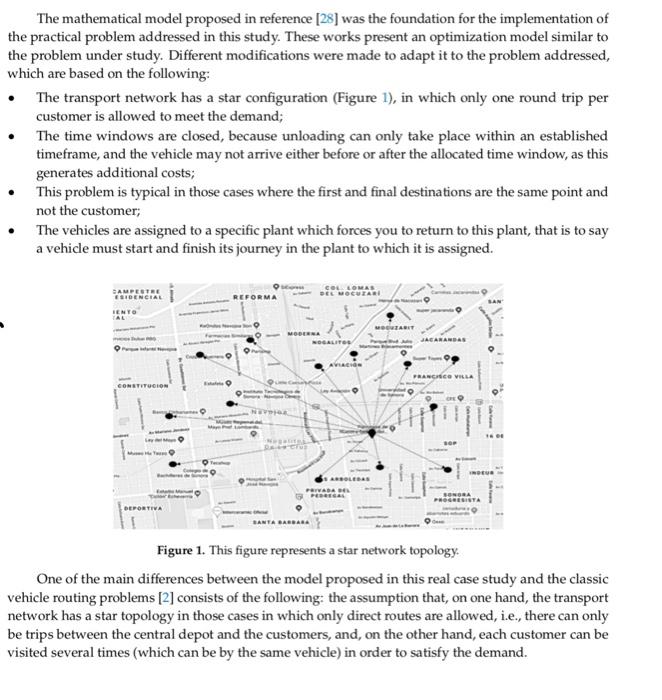
1. Objective The objective consists of minimizing the total integrated transport cost by the sum of the costs of the trip, which includes the costs generated, whether due to arriving late or early to the customer, the cost of the fuel used to move from the central depot to each customer and vice versa, and meeting the demands of each customer while considering time windows, vehicle capacity, and distribution center restrictions, and duration of the workday. 2 Justification In reference (25), the importance of the transport and its impact on the company's logistics distribution systems are weighted, so the proper use of the available logistical resources is at the center of most distribution route design problems. The cost associated with the transportation process represents between 10% and 20% of the total cost of the products (26), The work presented in reference (27) establishes that land transport represents 75% of available transport utilized, making it the most widely used, followed by rail with 17%, maritime with 7%, and air with 1%. Among its main advantages are its door-to-door service, its flexibility due to a wide variety of adapted vehicles of all load types and volumes, and the speed and facility with which it can be coordinated with other means of transport. The main disadvantage is that it must be limited to the weight and volume of the load to be moved. 3. Problem Statemen In many organizations, the planning of transport and distribution activities represents a serious decision-making problem. This situation has become increasingly important due to the contribution of distribution costs in the total product costs. Many enterprises require a fleet of vehicles for the collection and/or delivery of products within a distribution network. The efficient programming and use of said fleet is the main problem in the Sustainability 2020, 12, 63 5 of 10 majority of transport problems. Distribution area managers specifically ask themselves, how many from which plant, and what capacity should the vehicles be to satisfy the demand of each customer at a minimal cost? This question is difficult to answer due to the substantial number of possible combinations among the mix of fleet and routes, this is at the heart of how the proposed model has been implemented in this work [28]. There are currently two main variables that the business of cargo transport (VRP) focuses on. The first is the cost of fuel and the reduction in contaminant particle emissions into the environment Therefore, cargo truck manufacturers have focused their attention over the last decade on technological development and innovation to achieve greater fuel consumption efficiency, seeking to gain a competitive advantage over rivals in the market that benefits the enterprise's profitability. To increase truck carrying capacity, automotive equipment for more than 30 tons is being designed, with different interconnected equipment for greater load capacity and consolidation, thus maximizing the movement of goods in long hauls and reducing the transport cost [29]. The mathematical model proposed in reference [28] was the foundation for the implementation of the practical problem addressed in this study. These works present an optimization model similar to the problem under study. Different modifications were made to adapt it to the problem addressed, which are based on the following: The transport network has a star configuration (Figure 1), in which only one round trip per customer is allowed to meet the demand; The time windows are closed, because unloading can only take place within an established timeframe, and the vehicle may not arrive either before or after the allocated time window, as this generates additional costs; This problem is typical in those cases where the first and final destinations are the same point and not the customer; The vehicles are assigned to a specific plant which forces you to return to this plant, that is to say a vehicle must start and finish its journey in the plant to which it is assigned. SAM ESIDENCIAL COLLOMAS DEL MOCHIARI REFORMA MTARIT MORE JACARANDAS PRANCHCO VILLA ARDLESS PRIVADA DEPORTIVA BARA Figure 1. This figure represents a star network topology One of the main differences between the model proposed in this real case study and the classic vehicle routing problems [2] consists of the following: the assumption that, on one hand, the transport network has a star topology in those cases in which only direct routes are allowed, i.e., there can only be trips between the central depot and the customers, and, on the other hand, each customer can be visited several times (which can be by the same vehicle) in order to satisfy the demand. 1 Set of clients P = Set of plants 1 = Set of travels K = Set of vehicles i = Index corresponding to customers i el = 10,1,2,3,... p = Index corresponding to plants p P = (1,2,3,...,P) i = Index corresponding to travelsj ] = 11,2,3,...) k = Index corresponding to tehiclesk K = 11,2,3,...,K} E; = Window start time for customer ie ! Li - Window end time for customer i El Cp Cost of a trip to customer i from plant p;i EI, PEP Cdo = Cost for arriving late to customer i from plant p;iel, pep = Cost for arriving early to customer i from plant prie l.pep D. - Customer i demand; i el in = Travel time to customer i from plant p;i I, PEP Qip = Capacity of crickek from plant p;k K, PEP Decision variables 1 1 If customer i is visited by vehicle kon trip i from plant p otherwise Syx Schedule in telich each vehicle k must leave to complete each trip from each plant p W: Vehiclek waiting time at customer i on trip from plant p ExVehicle k delay time at customer i on trip from plant p Objective Function and Restrictions The objective of the problem consists of determining a set of routes to be followed considering a fleet of heterogeneous vehicles that depart from one or more central depots or warehouses intending to satisfy the demand of various geographically dispersed customers, minimizing the total cost of product transport The resulting mathematical model in mixed-integer linear programming is presented below. Equation (1) calculates the total transport cost, which includes the cost for visiting the customer, as well as the costs for deviations or non-compliance within the time windows for the different customers in the distribution network Objective function: Min X - ,WA +ca, (1) = { . PA a To ensure that for any trip, a vehicle is exactly in the plant (customer (0)) or visiting a customer, the following restriction is established (2) Xopx + xpx = 1, pe P.je), KEK 100 An obligatory restriction in the majority of routing problems is that of meeting customer demand, which is established with Restriction (3), expressed by the following equation: Q.Xmj 2 dj i EI, IU 101 (3) PA Sustainability 2020, 12, 63 7 of 10 If a vehicle is used, the time-of-use conditions must be established as well as the departure time for each trip to be made. It is also established that a trip can only begin once vehicle k has retumed to the depot after its previous trip. Restriction (4) is established for this purpose via the following expression: Su+1.4 2 Syx+ 20. Xipje PEP.; ),KEK (4) This ensures that if on any trip, the customer is not visited (Xpjk = 0) then there is no cost for arriving early, given that (W* = 0), otherwise, the time violation is calculated as standard, depending on Restriction (5) given by the following expression: WAZEX-(S.x+0yXipik) Vi+O, pe P.; ),kek (5) To estimate the cost of arriving after each customer's closing time window, Restriction (6) is established, given by the following expression: W(Sx+0yXwm) - L, -M(1-Xw*) Vi#O, pe P.) /kek (6) Here, M refers to a large positive integer to full fill (M25px-L.). It must be clarified that in (5) and (6) >0 only for Spx +00 only for Spx + Op> L, so for E, SL always Depending on the characteristics of the variables defined in the model, binary (0.1) and continuous variables are established. This situation is established through Restriction (7), given by the following expression: Xp4 10,1), W (7) a W+ -0. W by Six 20