

Question: g . Bold cells B 3 :E 3 . h . Apply the Accounting Number Format with 0 digits after the decimal to cells B
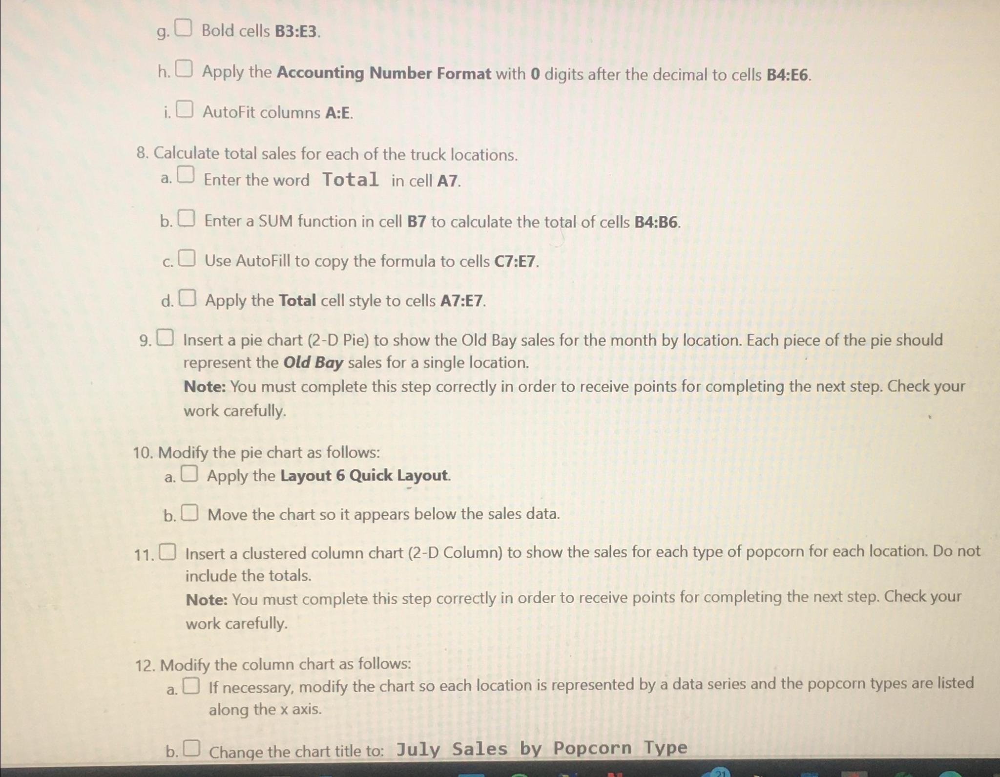
g Bold cells B:E
h Apply the Accounting Number Format with digits after the decimal to cells B:E
i AutoFit columns A:E
Calculate total sales for each of the truck locations.
a Enter the word Total in cell A
b Enter a SUM function in cell B to calculate the total of cells B:B
c Use AutoFill to copy the formula to cells C:E
d Apply the Total cell style to cells A:E
Insert a pie chart D Pie to show the Old Bay sales for the month by location. Each piece of the pie should represent the Old Bay sales for a single location.
Note: You must complete this step correctly in order to receive points for completing the next step. Check your work carefully.
Modify the pie chart as follows:
a Apply the Layout Quick Layout.
b Move the chart so it appears below the sales data.
Insert a clustered column chart D Column to show the sales for each type of popcorn for each location. Do not include the totals.
Note: You must complete this step correctly in order to receive points for completing the next step. Check your work carefully.
Modify the column chart as follows:
a If necessary, modify the chart so each location is represented by a data series and the popcorn types are listed along the axis.
b Change the chart title to: July Sales by Popcorn Type
Step by Step Solution
There are 3 Steps involved in it
1 Expert Approved Answer
Step: 1 Unlock

Question Has Been Solved by an Expert!
Get step-by-step solutions from verified subject matter experts
Step: 2 Unlock
Step: 3 Unlock