g$.$

Copy the formula in cell D$4$ to cells D$5$:D$10.$

h$.$

Click the Summary sheet tab, select cell A$5,$ and create a $3$D reference to cell D$4$ on the Technicians sheet.

i$.$

Copy the formula and preserve the borders.

Use SUMIFS to total number of patients by procedure and technician.

a$.$

Click the Summary sheet tab and select cell $C5.$

b$.$

Use the SUMIFS function with an absolute reference to cells $$D$$$5$:$$D$$$41$ on the Procedures sheet as the

Sum$\_$range argument.

$$

The Criteria$\_$range$1$ argument is an absolute reference to the image type column on the Procedures

sheet, cells $E$$5$:$$41.$

$$

The Criteria$1$ argument is a relative reference to cell $B5$ on the summary sheet.

$$

The Criteria$\_$range$2$ argument is an absolute reference to the technician names column on the

Procedures sheet.

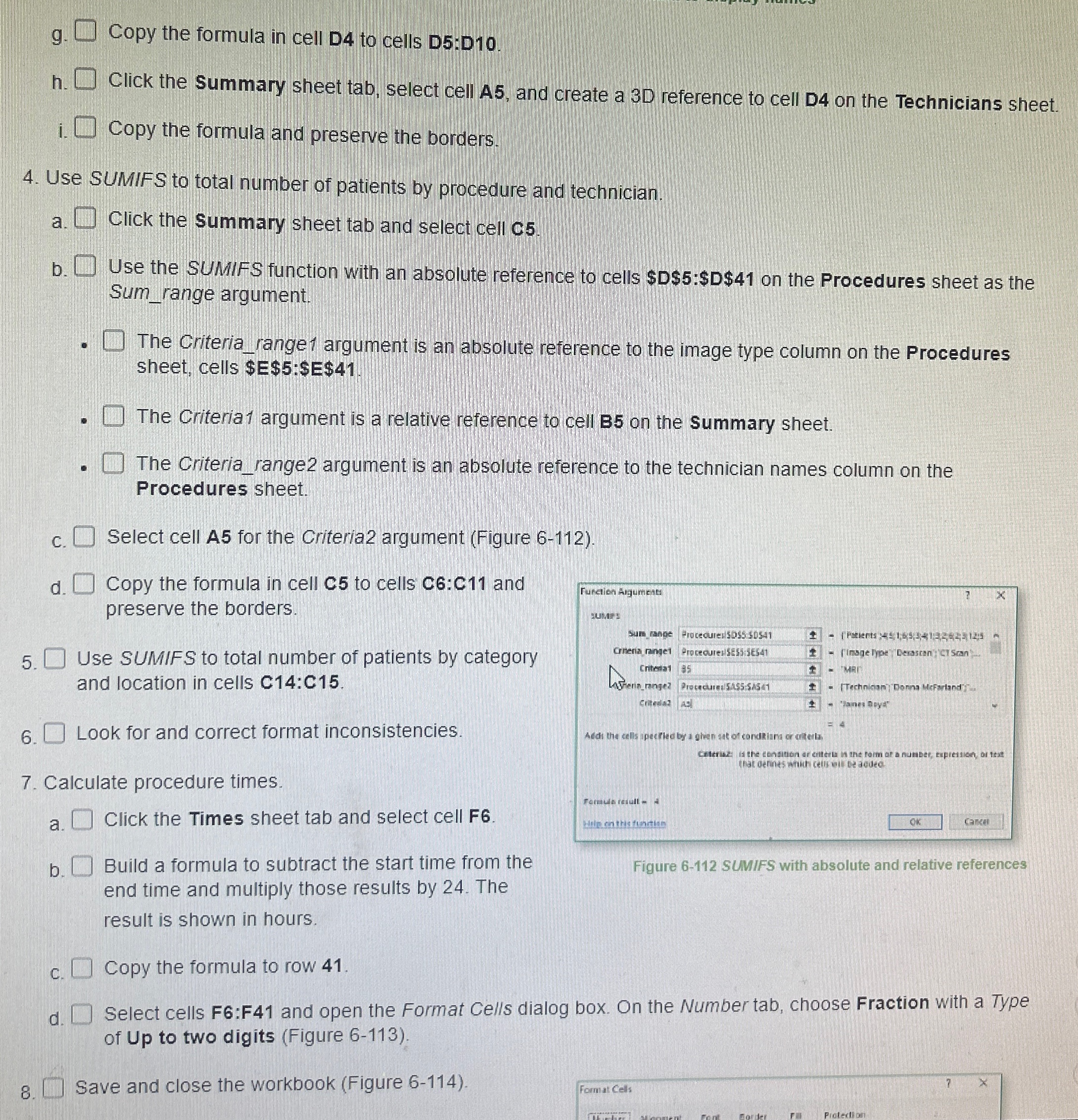
c$.$

Select cell A$5$ for the Criteria$2$ argument $($Figure $6-112).$

d$.$

Copy the formula in cell C$5$ to cells C$6$:C$11$ and

preserve the borders.

Use SUMIFS to total number of patients by category

and location in cells C$14$:C$15.$

Look for and correct format inconsistencies.

Calculate procedure times.

a$.$

Click the Times sheet tab and select cell F$6.$

b$.$

Build a formula to subtract the start time from the

end time and multiply those results by $24.$ The

Figure $6-112$ SUMIFS with absolute and relative references

result is shown in hours.

c$.$

Copy the formula to row $41.$

d$.$

Select cells F$6$:F$41$ and open the Format Cells dialog box. On the Number tab, choose Fraction with a Type

of Up to two digits $($Figure $6-113).$

Save and close the workbook $($Figure $6-114).$