Summarize Data Using Linked External References

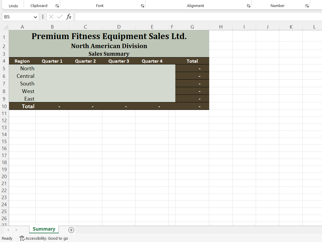
1. Open PFSalesSum.xlsx and save it with the name 4-PFSalesSum.

2. Open PFQ1.xlsx, PFQ2.xlsx, PFQ3.xlsx, and PFQ4.xlsx.

3. Tile all the open workbooks. Hint: With 4-PFSalesSum as the active workbook, use the Arrange All button on the View tab.

4. Starting in cell B5 in 4-PFSalesSum, create formulas to populate the cells in column B by linking to the appropriate source cells in PFQ1. Hint: After creating the first formula, edit the entry in cell B5 to use a relative reference to the source cell (instead of an absolute reference) so you can copy the formula in cell B5 to the range B6:B9.

5. Create formulas to link to the appropriate source cells for the second-, third-, and fourth-quarter sales.

6. Close the four quarterly sales workbooks. Click Dont Save if prompted to save changes.

7. Maximize 4-PFSalesSum.

8. Make cell B5 the active cell and then break the link to PFQ1.xlsx.

9. Save, preview, and then close 4-PFSalesSum.xlsx.

Create and Customize Sparklines

1. Open 4-PFSalesSum.xlsx and enable the content. Do not update the links.

2. Save the workbook with the name 4-PFSalesSum-6.

3. Select the range H5:H9 and insert line-type Sparklines referencing the range B5:E9.

4. Show the high point on each line.

5. Change the Sparkline color to dark blue (ninth option in the Standard Colors section).

6. Change the width of column H to 21 characters and type the label Region Sales by Quarter in cell H4.

7. Change the page layout to Landscape orientation and then preview the worksheet.

8. Save and then close 4-PFSalesSum-6.xlsx

=