Give Detailed Steps to solve These excel problems

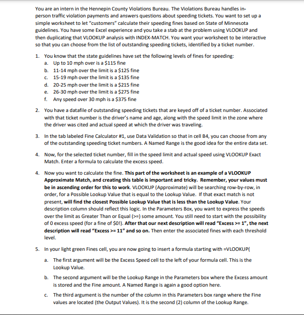
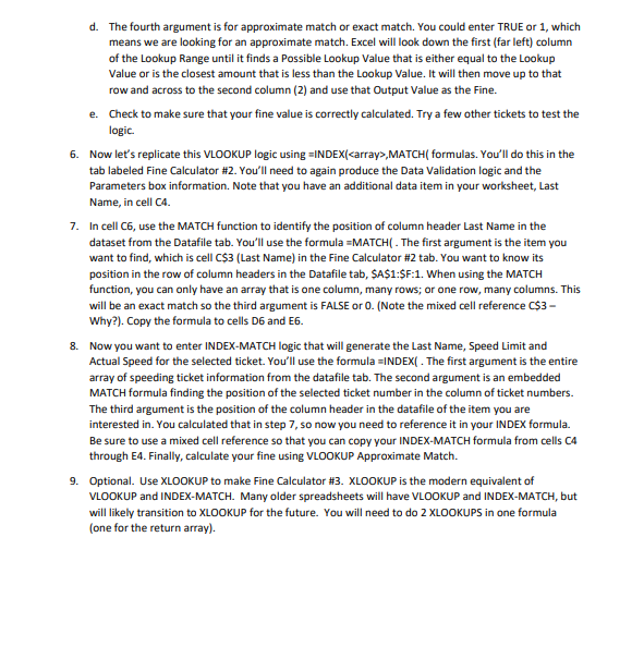
You are an intern in the Hennepin County Violations Bureau. The Violations Bureau handles inperson traffic violation payments and answers questions about speeding tickets. You want to set up a simple worksheet to let "customers" calculate their speeding fines based on State of Minnesota guidelines. You have some Excel experience and you take a stab at the problem using VLOOKUP and then duplicating that VLOOKUP analysis with INDEX-MATCH. You want your worksheet to be interactive so that you can choose from the list of outstanding speeding tickets, identified by a ticket number. 1. You know that the state guidelines have set the following levels of fines for speeding: a. Up to 10mph over is a $115 fine b. 11-14 mph over the limit is a $125 fine c. 1519mph over the limit is a $135 fine d. 20-25 mph over the limit is a $215 fine e. 26-30 mph over the limit is a $275 fine f. Any speed over 30mph is a $375 fine 2. You have a datafile of outstanding speeding tickets that are keyed off of a ticket number. Associated with that ticket number is the driver's name and age, along with the speed limit in the zone where the driver was cited and actual speed at which the driver was traveling. 3. In the tab labeled Fine Calculator \#1, use Data Validation so that in cell B4, you can choose from any of the outstanding speeding ticket numbers. A Named Range is the good idea for the entire data set. 4. Now, for the selected ticket number, fill in the speed limit and actual speed using VLOOKUP Exact Match. Enter a formula to calculate the excess speed. 4. Now you want to calculate the fine. This part of the worksheet is an example of a VLOOKUP Approximate Match, and creating this table is important and tricky. Remember, your values must be in ascending order for this to work. VLOOKUP (Approximate) will be searching row-by-row, in order, for a Possible Lookup Value that is equal to the Lookup Value. If that exact match is not present, will find the closest Possible Lookup Value that is less than the Lookup Value. Your description column should reflect this logic. In the Parameters Box, you want to express the speeds over the limit as Greater Than or Equal (>=) some amount. You still need to start with the possibility of 0 excess speed (for a fine of $0 !). After that our next description will read "Excess >=1, the next description will read "Excess >=11" and so on. Then enter the associated fines with each threshold level. 5. In your light green Fines cell, you are now going to insert a formula starting with =VLOOKUP( a. The first argument will be the Excess Speed cell to the left of your formula cell. This is the Lookup Value. b. The second argument will be the Lookup Range in the Parameters box where the Excess amount is stored and the Fine amount. A Named Range is again a good option here. c. The third argument is the number of the column in this Parameters box range where the Fine values are located (the Output Values). It is the second (2) column of the Lookup Range. d. The fourth argument is for approximate match or exact match. You could enter TRUE or 1, which means we are looking for an approximate match. Excel will look down the first (far left) column of the Lookup Range until it finds a Possible Lookup Value that is either equal to the Lookup Value or is the closest amount that is less than the Lookup Value. It will then move up to that row and across to the second column (2) and use that Output Value as the Fine. e. Check to make sure that your fine value is correctly calculated. Try a few other tickets to test the logic. 6. Now let's replicate this VLOOKUP logic using =INDEX (,MATCH( formulas. You'll do this in the tab labeled Fine Calculator \#2. You'll need to again produce the Data Validation logic and the Parameters box information. Note that you have an additional data item in your worksheet, Last Name, in cell C4. 7. In cell C6, use the MATCH function to identify the position of column header Last Name in the dataset from the Datafile tab. You'll use the formula =MATCH ( . The first argument is the item you want to find, which is cell C$3 (Last Name) in the Fine Calculator $2 tab. You want to know its position in the row of column headers in the Datafile tab, \$A\$1:\$F:1. When using the MATCH function, you can only have an array that is one column, many rows; or one row, many columns. This will be an exact match so the third argument is FALSE or 0 . (Note the mixed cell reference C$3 Why?). Copy the formula to cells D6 and E6. 8. Now you want to enter INDEX-MATCH logic that will generate the Last Name, Speed Limit and Actual Speed for the selected ticket. You'll use the formula =INDEX( . The first argument is the entire array of speeding ticket information from the datafile tab. The second argument is an embedded MATCH formula finding the position of the selected ticket number in the column of ticket numbers. The third argument is the position of the column header in the datafile of the item you are interested in. You calculated that in step 7, so now you need to reference it in your INDEX formula. Be sure to use a mixed cell reference so that you can copy your INDEX-MATCH formula from cells C4 through E4. Finally, calculate your fine using VLOOKUP Approximate Match. 9. Optional. Use XLOOKUP to make Fine Calculator \#3. XLOOKUP is the modern equivalent of VLOOKUP and INDEX-MATCH. Many older spreadsheets will have VLOOKUP and INDEX-MATCH, but will likely transition to XLOOKUP for the future. You will need to do 2 XLOOKUPS in one formula (one for the return array)