Good afternoon,

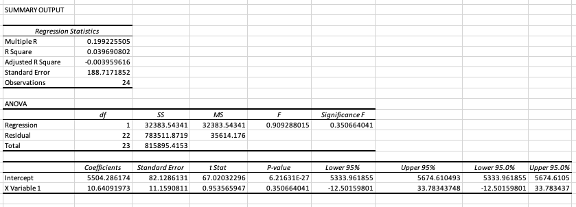
I am having difficulties running the regression statistics report from the below. I used the deseasonalized sales figures against the period time which (the column titled "Observation") for the regression. However my numbers are different from the textbook example. Please see the excel report and Textbook example in the below and let me know what variables I need to use against the period time to get the same exact regression statistics that is reference in the textbook.

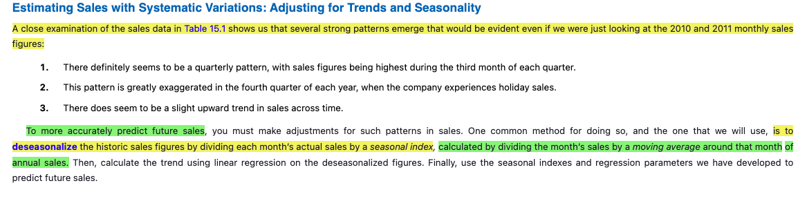
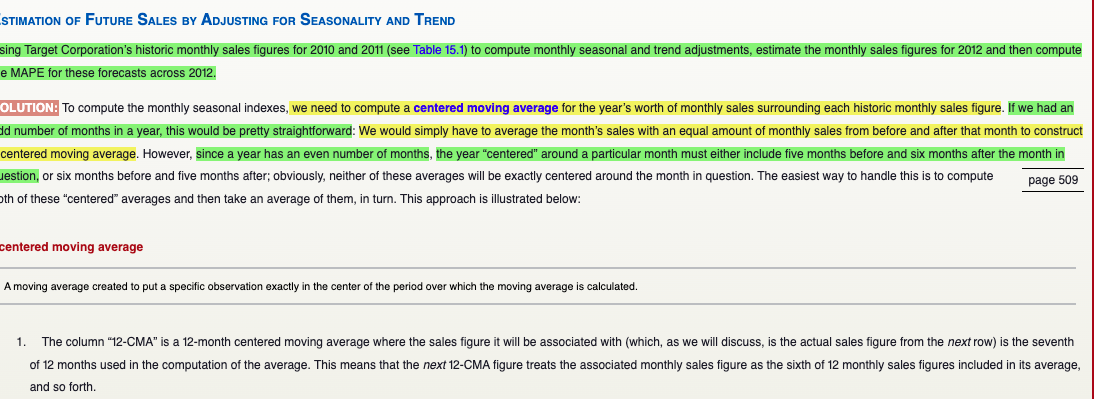
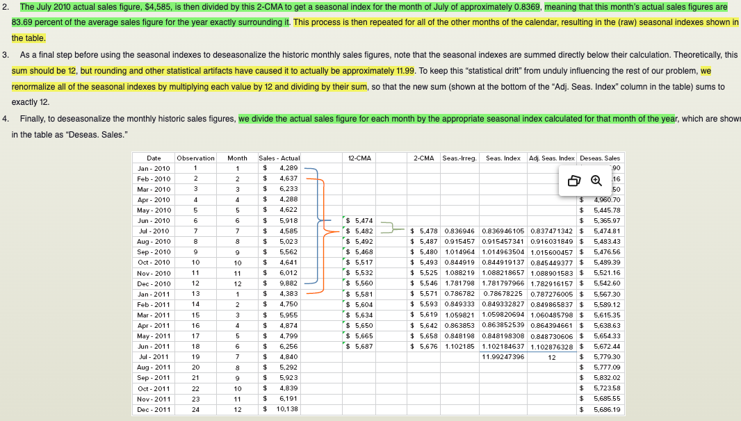
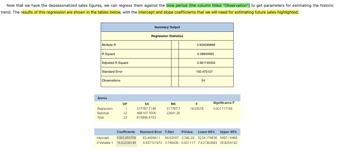
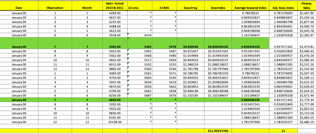
Estimating Sales with Systematic Variations: Adjusting for Trends and Seasonality A close examination of the sales data in Table 15.1 shows us that several strong patterns emerge that would be evident even if we were just looking at the 2010 and 2011 monthly sales figures: 1. There definitely seems to be a quarterly pattern, with sales figures being highest during the third month of each quarter. 2. This pattern is greatly exaggerated in the fourth quarter of each year, when the company experiences holiday sales. 3. There does seem to be a slight upward trend in sales across time. To more accurately predict future sales, you must make adjustments for such patterns in sales. One common method for doing so, and the one that we will use, is to deseasonalize the historic sales figures by dividing each month's actual sales by a seasonal index, calculated by dividing the month's sales by a moving average around that month of annual sales. Then, calculate the trend using linear regression on the deseasonalized figures. Finally, use the seasonal indexes and regression parameters we have developed to predict future sales.STIMATION OF FUTURE SALES BY ADJUSTING FOR SEASONALITY AND TREND sing Target Corporation's historic monthly sales figures for 2010 and 2011 (see Table 15.1) to compute monthly seasonal and trend adjustments, estimate the monthly sales figures for 2012 and then compute e MAPE for these forecasts across 2012. OLUTION: To compute the monthly seasonal indexes, we need to compute a centered moving average for the year's worth of monthly sales surrounding each historic monthly sales figure. If we had an Id number of months in a year, this would be pretty straightforward: We would simply have to average the month's sales with an equal amount of monthly sales from before and after that month to construct centered moving average. However, since a year has an even number of months, the year "centered" around a particular month must either include five months before and six months after the month in estion, or six months before and five months after; obviously, neither of these averages will be exactly centered around the month in question. The easiest way to handle this is to compute page 509 oth of these "centered" averages and then take an average of them, in turn. This approach is illustrated below: centered moving average A moving average created to put a specific observation exactly in the center of the period over which the moving average is calculated. 1. The column "12-CMA" is a 12-month centered moving average where the sales figure it will be associated with (which, as we will discuss, is the actual sales figure from the next row) is the seventh of 12 months used in the computation of the average. This means that the next 12-CMA figure treats the associated monthly sales figure as the sixth of 12 monthly sales figures included in its average, and so forth.. The July 2010 actual sales figure, $4,585, is then divided by this 2-CMA to get a seasonal index for the month of July of approximately 0.8369, meaning that this month's actual sales figures are 83.69 percent of the average sales figure for the year exactly surrounding it. This process is then repeated for all of the other months of the calendar, resulting in the (raw) seasonal indexes shown in the table. 3. As a final step before using the seasonal indexes to deseasonalize the historic monthly sales figures, note that the seasonal indexes are summed directly below their calculation. Theoretically, this sum should be 12, but rounding and other statistical artifacts have caused it to actually be approximately 11.99. To keep this "statistical drift" from unduly influencing the rest of our problem, we renormalize all of the seasonal indexes by multiplying each value by 12 and dividing by their sum, so that the new sum (shown at the bottom of the "Adj. Seas. Index" column in the table) sums to exactly 12. 4. Finally, to deseasonalize the monthly historic sales figures, we divide the actual sales figure for each month by the appropriate seasonal index calculated for that month of the year, which are show in the table as "Deseas. Sales." Date Observation Month Sales - Actual 12-CMA 2-CMA Seas-Irreg. Seas. Index Adj. Seas. Index Deseas. Sales Jan - 2010 $ 4.289 Feb - 2010 2 2 4.637 16 Mar - 2010 3 6.233 50 Apr - 2010 4 4 4.288 $ 4,960.70 May - 2010 5 4.622 5,445.78 Jun - 2010 6 5.918 $ 5,474 $ 5.365.97 Jul - 2010 7 4.585 $ 5,482 $ 5,478 0.836946 0.836946105 0.837471342 $ 5,474.81 Aug - 2010 8 8 5.023 $ 5.492 $ 5.487 0.915457 0.915457341 0.916031849 $ 5,483.43 Sep - 2010 9 5,562 $ 5.468 $ 5,480 1.014964 1.014963504 1.015600457 $ 5,476.56 Oct - 2010 10 10 4,641 $ 5.517 $ 5,493 0.844919 0.844919137 0.845449377 $ 5,489.39 Nov - 2010 11 6,012 $ 5.532 $ 5.525 1.088219 1.088218657 1.088901583 $ 5,521.16 Dec - 2010 12 12 9.882 $ 5.560 $ 5.546 1.781798 1.781797966 1.782916157 $ 5,542.60 Jan - 2011 13 1 4,383 $ 5.581 $ 5.571 0.786782 0.78678225 0.787276005 $ 5,567.30 Feb - 2011 14 2 4,750 $ 5.604 $ 5.593 0.849333 0.849332827 0.849865837 $ 5,589.12 Mar - 2011 15 3 5,955 $ 5.634 $ 5.619 1.059821 1.059820694 1.060485798 $ 5.615.35 Apr - 2011 16 4 4.874 $ 5.650 $ 5.642 0.863853 0.863852539 0.864394661 $ 5,638.63 May - 2011 17 5 4.799 $ 5.665 $ 5.658 0.848198 0.848198308 0.848730606 $ 5,654.33 Jun - 2011 18 6 6.256 $ 5.687 $ 5.676 1.102185 1.102184637 1.102876328 $ 5,672.44 Jul - 2011 19 7 $ 4.840 11.99247396 12 $ 5,779.30 Aug - 2011 20 8 5,292 $ 5,777.09 Sep - 2011 21 5,923 5,832.02 Oct - 2011 22 10 4.839 5.723.58 Nov - 2011 23 11 6.191 5.685.55 Dec - 2011 24 12 10.138 $ 5,686.19Now that we have the deseasonalized sales figures, we can regress them against the time period (the column titled "Observation") to get parameters for estimating the historic trend. The results of this regression are shown in the tables below, with the intercept and slope coefficients that we will need for estimating future sales highlighted. Summary Output Regression Statistics Multiple R 0.624095866 R Square 0.38949565 Adjusted R Square 0.361745452 Standard Error 150.470127 Observations 24 Anova DF SS MS Significance F Regression 317787.7149 317787.7 14.03578 0.001 117156 Residual 22 498 107.7005 22641.26 Total 23 815895.4153 Coefficients Standard Error T-Stat P-Value Lower 95% Upper 95% Intercept 5365.659759 63.400661 1 84.63097 3.74E-29 5234.174836 5497.14468 XVariable 1 16.62339145 4.437121973 3.746436 0.001117 7.421363693 25.8254192Sales - Actual Deseas, Date Observation Month 2010 & 2011 12-cma 2-CMA Seas-Irreg Seas Index Average Seasonal Index Adj. Seas, Index Sales January 00 - - - . . . . . . .- - - - - - 1 1289.00 0.78678225 0.787276005 $5,447.90 - -L- January 00 wiNi 1637.00 0.849332827 0.849865837 $5,456.16 - - - -. . . . .!...... win January 00 6233.00 1.059820694 1.060485798 $5,877.50 January 00 A 4288.00 0.863852539 0.864394661 $4,960.70 - -- January 00 4622.00 0.848198308 J- --L-. 0.848730606 January 00 5918.00 5474: 1.102184637 1.102876328 $5,365.97 January 00 1585.00 5482: 5478 $0.836946 $0.836946105 0.836946105 0.837471342 $5,474.81 January 00 : LD : 00 : 4 5023.00 5492; 5487: 50.915457 $0.915457341 0.915457341 0.916031849 $5,483.43 5: :0014 January 00 5562.00 5468 5480: $1.014964 $1.014963504 1.014963504 1.015600457 -L-T $5,476.56 January 00 10 4641.00 5517; 5493; 50.844919 50.844919137 D.844919137 0.845449377 $5,489.39 - - - - . . . . . . . . . . . . . January 00 6012.00 5532: 5525: $1.088219 $1.088218657 1.088218657 - - -. . . ...!. - - - - - - - -- - - -. .. ...... 1.088901583 $5,521.16 January 00 9882.00 5560; 5546: $1.781798 $1.781797966 1.781797966 1.782916157 $5,542.60 January 00 1383.00 5581 ; 5571: 50.786782 50.786782250 0.78678225 0.787276005 $5,567.30 January 00 4750.00 5604; 5593 : 50.849333 - - - - - - -. . . . .. $0.849332827 0.849332827 --. . . . .. . ... . ....... 0.849865837 $5,589.12 January 00 5955.00 5634: 5619; $1.059821 $1.059820694 1.059820694 - - - . .- - - . . . . .. I- - - - - - - . . . . . . ... - --- - - - - - ---........ 1.060485798 $5,615.35 January 00 4874.00 5650; 5642: 50.863853 $0.863852539 0.863852539 0.864394661 $5,638.63 - - - - - - - -- .- -. January 00 1799.00 5665: 5658: 50.848198 $0.848198308 0.848198308 0.848730606 $5,654.33 -L- - - - - - - 4- - - - - - -4- -. -;- January 00 6256.00 5687 : 5676: $1.102185 $1.102184637 1.102184637 1.102876328 $5,672.44 100 1840.00 0.836946105 0.837471342 $5,779.30 January 00 5292.00 - - - - - - - - . . .. 0.915457341 -.... .... . .. ..-..... 0.916031849 $5,777.09 January 00 5923.00 1.014963504 1.015600457 - - - - - - - - - - - - - - $5,832.02 January 00 10 10 1839.00 0.844919137 --............. $5,723.58 -- - 0.845449377 January 00 11 11 6191.00 1.088218657 1.088901583 $5,685.55 January 00 17 10138.00 1.781797966 1.782916157 $5,686.19 -'- - -. ... . . . . . ... $11.99247396SUMMARY OUTPUT Regression Statistics Multiple R 0.199225505 R Square 0.039690802 Adjusted R Square -0.003959616 Standard Error 188.7171852 Observations 24 ANOVA df SS MS F Significance F Regression 32383.54341 32383.54341 0.909288015 0.350664041 Residual 22 783511.8719 35614.176 Total 23 815895.4153 Coefficients Standard Error t Stat P-value Lower 95% Upper 95% Lower 95.0% Upper 95.0% Intercept 5504.286174 82.1286131 67.02032296 6.21631E-27 5333.961855 5674.610493 5333.961855 5674.6105 X Variable 1 10.64091973 11.1590811 0.953565947 0.350664041 -12.50159801 33.78343748 -12.50159801 33.783437