H E L P

how could you need more information? the formula is right there on page 1

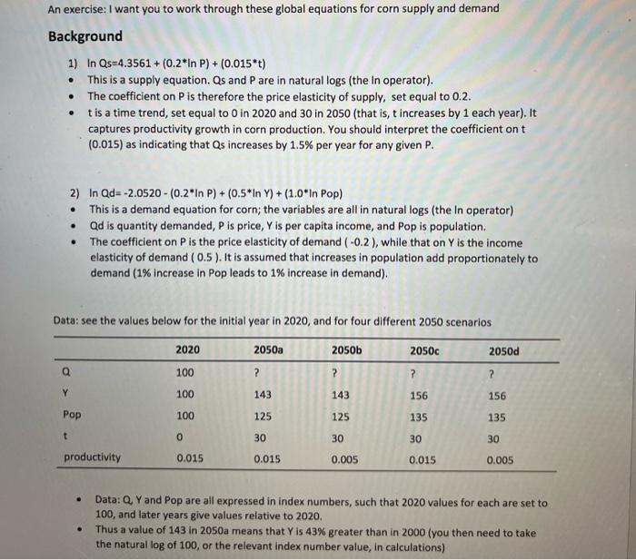
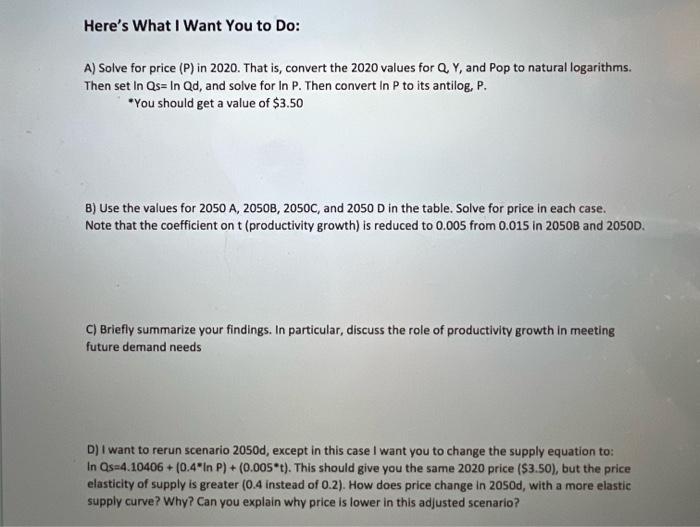
An exercise: I want you to work through these global equations for corn supply and demand Background 1) lnQs=4.3561+(0.2lnP)+(0.015t) - This is a supply equation. Qs and P are in natural logs (the In operator). - The coefficient on P is therefore the price elasticity of supply, set equal to 0.2. - t is a time trend, set equal to 0 in 2020 and 30 in 2050 (that is, t increases by 1 each year). It captures productivity growth in corn production. You should interpret the coefficient on t (0.015) as indicating that Q increases by 1.5% per year for any given P. 2) In Qd =2.0520(0.2lnP)+(0.5lnY)+(1.0lnPp) - This is a demand equation for corn; the variables are all in natural logs (the in operator) - Qd is quantity demanded, P is price, Y is per capita income, and Pop is population. - The coefficient on P is the price elasticity of demand (0.2), while that on Y is the income elasticity of demand (0.5). It is assumed that increases in population add proportionately to demand ( 1% increase in Pop leads to 1% increase in demand). Data: see the values below for the initial year in 2020, and for four different 2050 scenarios - Data: Q Y and Pop are all expressed in index numbers, such that 2020 values for each are set to 100 , and later years give values relative to 2020. - Thus a value of 143 in 2050 means that Y is 43% greater than in 2000 (you then need to take the natural log of 100 , or the relevant index number value, in calculations) A) Solve for price (P) in 2020. That is, convert the 2020 values for Q Y, and Pop to natural logarithms. Then set lnQs=lnQd, and solve for lnP. Then convert lnP to its antilog, P. "You should get a value of $3.50 B) Use the values for 2050A,2050B,2050C, and 2050D in the table. Solve for price in each case. Note that the coefficient on t (productivity growth) is reduced to 0.005 from 0.015 in 20508 and 2050D. C) Briefly summarize your findings. In particular, discuss the role of productivity growth in meeting future demand needs D) I want to rerun scenario 2050d, except in this case I want you to change the supply equation to: In Qs=4.10406 +(0.4lnP)+(0.005t). This should give you the same 2020 price ($3.50), but the price elasticity of supply is greater (0.4 instead of 0.2). How does price change in 2050d, with a more elastic supply curve? Why? Can you explain why price is lower in this adjusted scenario? An exercise: I want you to work through these global equations for corn supply and demand Background 1) lnQs=4.3561+(0.2lnP)+(0.015t) - This is a supply equation. Qs and P are in natural logs (the In operator). - The coefficient on P is therefore the price elasticity of supply, set equal to 0.2. - t is a time trend, set equal to 0 in 2020 and 30 in 2050 (that is, t increases by 1 each year). It captures productivity growth in corn production. You should interpret the coefficient on t (0.015) as indicating that Q increases by 1.5% per year for any given P. 2) In Qd =2.0520(0.2lnP)+(0.5lnY)+(1.0lnPp) - This is a demand equation for corn; the variables are all in natural logs (the in operator) - Qd is quantity demanded, P is price, Y is per capita income, and Pop is population. - The coefficient on P is the price elasticity of demand (0.2), while that on Y is the income elasticity of demand (0.5). It is assumed that increases in population add proportionately to demand ( 1% increase in Pop leads to 1% increase in demand). Data: see the values below for the initial year in 2020, and for four different 2050 scenarios - Data: Q Y and Pop are all expressed in index numbers, such that 2020 values for each are set to 100 , and later years give values relative to 2020. - Thus a value of 143 in 2050 means that Y is 43% greater than in 2000 (you then need to take the natural log of 100 , or the relevant index number value, in calculations) A) Solve for price (P) in 2020. That is, convert the 2020 values for Q Y, and Pop to natural logarithms. Then set lnQs=lnQd, and solve for lnP. Then convert lnP to its antilog, P. "You should get a value of $3.50 B) Use the values for 2050A,2050B,2050C, and 2050D in the table. Solve for price in each case. Note that the coefficient on t (productivity growth) is reduced to 0.005 from 0.015 in 20508 and 2050D. C) Briefly summarize your findings. In particular, discuss the role of productivity growth in meeting future demand needs D) I want to rerun scenario 2050d, except in this case I want you to change the supply equation to: In Qs=4.10406 +(0.4lnP)+(0.005t). This should give you the same 2020 price ($3.50), but the price elasticity of supply is greater (0.4 instead of 0.2). How does price change in 2050d, with a more elastic supply curve? Why? Can you explain why price is lower in this adjusted scenario