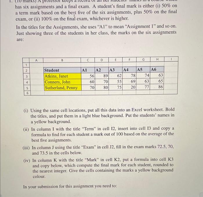
has six assignments and a final exam. A student's final mark is either (i) 50% on a term mark based on the bert five of the six assignments, plus 50% on the final exam, or (ii) 100% on the final exam, whichever is higher. In the titles for the Assignments, she uses "A1" to mean "Assignment 1" and so on. Just showing three of the students in her class, the marks on the six assignments are: (i) Using the same cell locations, put all this data into an Excel worksheet. Bold the titles, and put them in a light blue background. Put the students' names in a yellow background. (ii) In column I with the title "Term" in cell I2, insert into cell I3 and copy a formula to find for each student a mark out of 100 based on the average of the best five assignments. (iii) In column J using the title "Exam" in cell J2, fill in the exam marks 72.5,70, and 73.5 in the cells below. (iv) In column K with the title "Mark" in cell K2, put a formula into cell K3 and copy below, which compute the final mark for each student, rounded to the nearest integer. Give the cells containing the marks a yellow background colour. In your submission for this assignment you need to: (iii) In column J using the title "Exam" in cell J2, fill in the exam marks 72.5,70, and 73.5 in the cells below. (iv) In column K with the sitle "Mark" in cell K2, put a formula into cell K3 and copy below, which compute the final mark for each student, rounded to the nearest integer. Give the cells containing the marks a yellow background colour. In your submission for this assignment you need to: (a) Submit the range A1:K6 by importing the worksheet into Word or by converting it to pdf. 1 'In Excel, if printing to pdf, gridlines and row and column headings are made as follows. Go into Print, and at the bottom click on page setup. Click on Sheet, and then click on Gridlines and Row and column headings. Business 2400 , Winter 2023 , written by Dr. David M. Tulett 3 (b) Give the formula used in cell 13. (c) Give the formula used in cell K3