help me

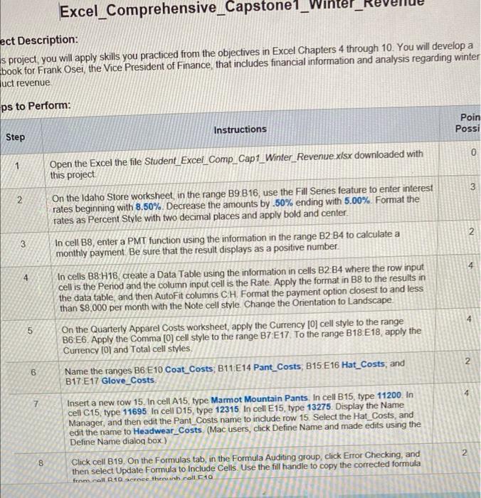
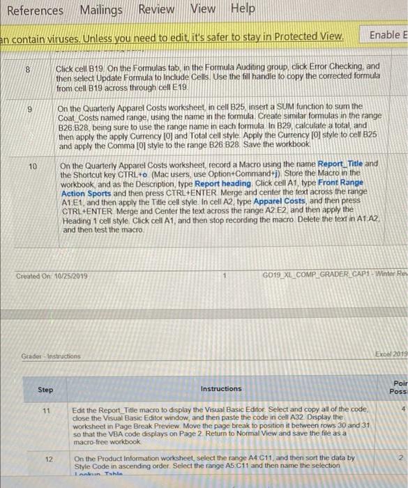
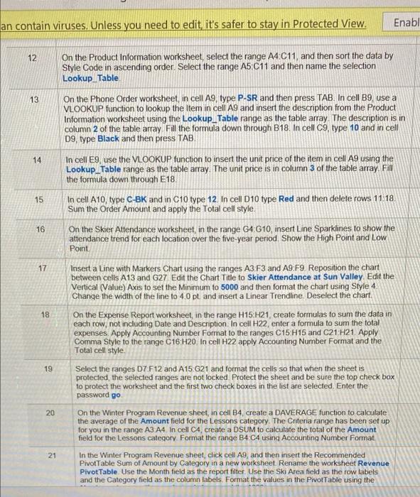
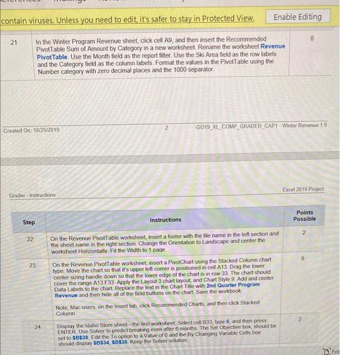
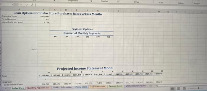
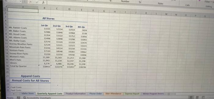
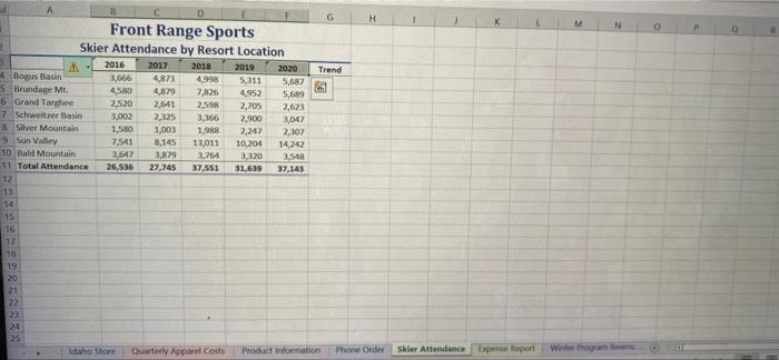
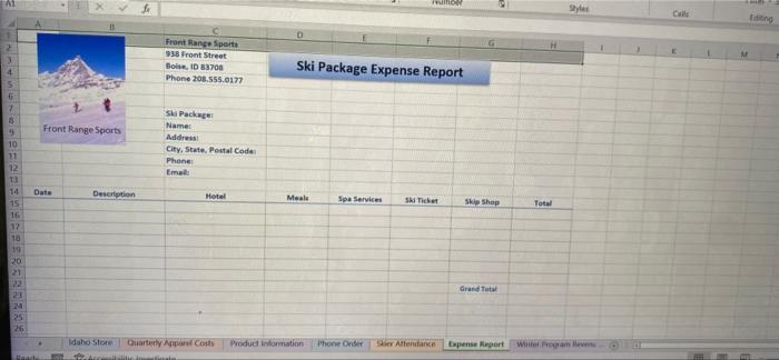
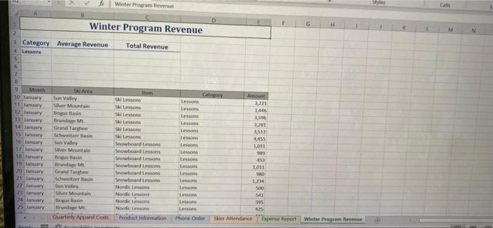
Excel_Comprehensive_Capstonel_Wint ect Description: s project, you will apply skills you practiced from the objectives in Excel Chapters 4 through 10. You will develop a book for Frank Osei, the Vice President of Finance that includes financial information and analysis regarding winter uct revenue ps to Perform: Poin Possi Instructions Step 0 1 3 2 2. 3 4 4 Open the Excel the file Student Excel_comp_Cap1_Winter_Revenue.xlsx downloaded with this project On the Idaho Store worksheet in the range B9 B16, use the Fill Series feature to enter interest rates beginning with 8.50%. Decrease the amounts by .50% ending with 5.00% Format the rates as Percent Style with two decimal places and apply bold and center In cell B8, enter a PMT function using the information in the range B2 B4 to calculate a monthly payment. Be sure that the result displays as a positive number In cells B8:H16, create a Data Table using the information in cells B2 B4 where the row input cell is the Period and the column input cell is the Rate. Apply the format in B8 to the results in the data table and then AutoFit columns CH. Format the payment option closest to and less than $8,000 per month with the Note cell style Change the Orientation to Landscape On the Quarterly Apparel Costs worksheet, apply the Currency [0] cell style to the range B6 E6. Apply the Comma [0] cell style to the range B7:E17 To the range B18E18. apply the Currency [0] and Total cell styles Name the ranges B6 E10 Coat_Costs: B11:E14 Pant_Costs, B15 E 16 Hat_Costs, and B17 E17 Glove_Costs Insert a new row 15. In cell A15, type Marmot Mountain Pants. In cell B15, type 11200. In cell C15, type 11695. In cell D15type 12315 In cell E15, type 13275. Display the Name Manager, and then edit the Pant_Costs name to include row 15 Select the Hat_Costs, and edit the name to Headwear_Costs (Mac users, click Define Name and made edits using the Define Name dialog box.) Click cell B19. On the Formulas tab, in the Formula Auditing group, click Error Checking, and then select Update Formula to Include Cells. Use the fill handle to copy the corrected formula 5 2 6 7 2 CO 8 from coll R10 acrece then roll 10 References Mailings Review View Help Enable E an contain viruses. Unless you need to edit it's safer to stay in Protected View. 8 Click cell B19. On the Formulas tab, in the Formula Auditing group, click Error Checking, and then select Update Formula to Include Cells. Use the fill handle to copy the corrected formula from cell B19 across through cell E19. 9 On the Quarterly Apparel Costs worksheet, in cell B25 insert a SUM function to sum the Coat Costs named range, using the name in the formula. Create similar formulas in the range B26,828, being sure to use the range name in each formula In B29, calculate a total and then apply the apply Currency [0] and Total cell style Apply the Currency [O] style to cell B25 and apply the Comma [0] style to the range B26 B28. Save the workbook, 10 On the Quarterly Apparel Costs worksheet, record a Macro using the name Report_Title and the Shortcut key CTRL+O (Mac users, use Option+Command+i) Store the Macro in the workbook, and as the Descnption, type Report heading Click cell A1, type Front Range Action Sports and then press CTRL+ENTER Merge and center the text across the range A1E1, and then apply the Title cell style. In cell A2 type Apparel Costs, and then press CTRL+ENTER Merge and Center the text across the range A2 E2 and then apply the Heading 1 cell style Click cell A1, and then stop recording the macro Delete the text in A1 A2 and then test the macro Created On: 10/25/2019 G019_XL_COMPGRADER_CAP Winter Re Grader Instructions Excel 2019 Step Instructions Poir Poss 11 Edit the Report_Title macro to display the Visual Basic Editor Select and copy all of the code, close the Visual Basic Editor window, and then paste the code in cell A32 Display the worksheet in Page Break Preview Move the page break to position it between rows 30 and 31 so that the VBA code displays on Page 2 Return to Normal View and save the file as a macro-free workbook 12 2. On the Product Information worksheet, select the range A4 C11, and then sort the data by Style Code in ascending order. Select the range A5 C11 and then name the selection Lankan Tahim an contain viruses. Unless you need to edit it's safer to stay in Protected View. Enabl 12 On the Product Information worksheet, select the range A4 C11 and then sort the data by Style Code in ascending order. Select the range A5 C11 and then name the selection Lookup_Table 13 On the Phone Order worksheet, in cell A9, type P-SR and then press TAB. In cell B9, use a VLOOKUP function to lookup the item in cell A9 and insert the description from the Product Information worksheet using the Lookup_Table range as the table array. The description is in column 2 of the table array Fill the formula down through B18. In cell C9, type 10 and in cell D9, type Black and then press TAB 14 In cell E9, use the VLOOKUP function to insert the unit price of the item in cell A9 using the Lookup_Table range as the table array. The unit price is in column 3 of the table array. Fill the formula down through E18 15 In cell A10, type C-BK and in C10 type 12. In cell D10 type Red and then delete rows 11 18. Sum the Order Amount and apply the Total cell style. On the Skier Attendance worksheet, in the range G4 G10, insert Line Sparklines to show the attendance trend for each location over the five-year period. Show the High Point and Low Point 16 17 18 19 Insert a Line with Markers Chart using the ranges A3 F3 and A9:F9 Reposition the chart between cells A13 and G27 Edit the Chart Title to Skier Attendance at Sun Valley Edit the Vertical (Value) Axis to set the Minimum to 5000 and then format the chart using Style 4 Change the width of the line to 40 pt and insert a Linear Trendline Deselect the chart. On the Expense Report worksheet, in the range H15 H21, create formulas to sum the data in each row, not including Date and Description In cell H22, enter a formula to sum the total expenses Apply Accounting Number Format to the ranges C15 H15 and C21H21. Apply Comma Style to the range C16 H20 In cell H22 apply Accounting Number Format and the Total cell style Select the ranges D7 F12 and A15 G21 and format the cells so that when the sheet is protected, the selected ranges are not locked Protect the sheet and be sure the top check box to protect the worksheet and the first two check boxes in the list are selected Enter the password go On the Winter Program Revenue sheet, in cell B4, create a DAVERAGE function to calculate the average of the Amount field for the Lessons category. The Criteria range has been set up for you in the range A3 A4 In cell C4, create a DSUM to calculate the total of the Amount field for the Lessons category. Format the range B4 C4 using Accounting Number Format In the Winter Program Revenue sheet, click cell Ag, and then insert the Recommended Pivot Table Sum of Amount by Category in a new worksheet. Rename the worksheet Revenue Pivot Table. Use the Month field as the report filter. Use the Ski Area field as the row labels and the Category field as the column labels. Format the values in the PivotTable using the 20 21 contain viruses. Unless you need to edit, it's safer to stay in Protected View. Enable Editing 8 21 In the Winter Program Revenue sheet, click cell A9, and then insert the Recommended Pivot Table Sum of Amount by Category in a new worksheet. Rename the worksheet Revenue Pivot Table. Use the Month field as the report filter. Use the Ski Area field as the row labels and the Category field as the column labels Format the values in the PivotTable using the Number category with zero decimal places and the 1000 separator 2 Created On 10/25/2019 G019_XL_COMP GRADER_CAP1 - Winter Revenue 10 Excel 2019 Project Grader - Instructions Points Possible Instructions Step 2 22 8 23 On the Revenue PivotTable worksheet, insert a footer with the file name in the left section and the sheet name in the right section Change the Orientation to Landscape and center the worksheet Horizontally Fit the Width to 1 page. On the Revenue PivotTable worksheet, insert a PivotChart using the Stacked Column chart type. Move the chart so that it's upper left comer is positioned in cell A13 Drag the lower center sizing handle down so that the lower edge of the chart is in row 33. The chart should cover the range A13 F33. Apply the Layout 3 chart layout and Chart Style 9. Add and center Data Labels to the chart Replace the text in the Chart Tide with 2nd Quarter Program Revenue and then hide all of the field buttons on the chart Save the workbook Note, Mac users on the Insert tab, click Recommended Charts, and then click Stacked Column Display the Idaho Store sheet-the first worksheet Select cell B33, type 6, and then press ENTER Use Solver to predict breaking even after 6 months The Set Objective box, should be set to $B$38. Edit the To option to a value of O and the By Changing Variable Cells box should display $B$34. $B$36. Keep the Solver solution 2 24 D Foc Number Loan Options for Idaho Store Purchase: Rates versus Months Molto 3950,000 Periodic 130 este per year WIN Payment Options Number of Monthly Payments 200 NO 120 LO 360 Projected Income Statement Model 1 2 S . $ 125.000 $137.500 1.250 $ 166,375 5183,013 52013343221.445 524.00 $17,057 MIN 1 Sales 313 Expenses Cosed to Idaho Store Quarterly Apparel Costs 119425 11.5 Production 1407 1221 173.1 Phone Onder Skor Attendance w M Number Filter B C D 2 H a 31 All Stores 4 5 1st Our 2nd Que 6 M. Rainier Coats 11155 12554 7 Mt Baker Coats 12456 11846 8 Mt Hood Coats 11354 11522 9 Mt. Adams Coats 11498 12898 10 Mt Baldy Coats 12570 11320 11 Stormy Weather Pants 12129 12221 12 Mountain Rain Pants 13226 14116 13 VenturePants 17110 TRER 14 Snowy River Pants 11220 12250 15 Women's Hats 11.183 16 Men's 11,23 11,234 17 Gloves 6,176 6,986 1 Total by Carter 116415 122226 19 20 21 Apparel Costs 22 Annual Costs for All Stores 22 24 Coat Corts 25 Mar Costs Idaho Store Quarterly Apparel Costs Lead Accessibilitimeste Srdar 12554 130 11752 13298 11119 12323 15218 19281 14358 11,213 12,147 10,146 131057 4th Or 1824 15 11856 11053 11424 13223 11316 19362 1449 11.1 11,199 12,248 130216 Product Information e Order Ser Alundance (sperme leport Winter D G 1 Front Range Action Sports Product List 2 3 4 Style Code 5 P SR 6 PMR 7 P.VI BC RR 9 C BK 10 C-HD 11 C-AD 12 13 14 15 16 17 18 19 20 Description Snowy River pant Mountain Rain pant Venture part ML Rainier coat Mt. Baker coat Mt. Hood coat MI Adams coat Unit Price $ 125.00 S 140.00 S 157.00 $ 116.00 $ 333.00 5 359.00 $ 325.00 Front Range Action Sports B E G H K D Front Range Action Sports Phone Order Form Customer Name Customer Number Order Dato 7 3 Item Description Quantity Color Unit Price Order Amount S 10 11 32 73 15 16 17 18 19 20 21 Totalt G K w N Trend A B Front Range Sports 2 Skier Attendance by Resort Location 3 2016 2017 2015 2019 2020 Bogus Basin 3,666 4,873 4.998 5,211 5,687 5 Brundage MI. 4,500 4,879 7,826 4,952 5,689 6 Grand Targhese 2,520 2,641 2,50 2,705 2,623 -7 Schweitzer Basin 3,002 7,325 3,366 2,900 3,04 8 Silver Mountain 1,580 1,003 1.988 2,247 2302 3 Sun Valley 7,541 8,145 13,011 10,204 14242 10 Bald Mountain 3,647 3,879 3,764 3,320 3548 11 Total Attendance 26,536 27,745 37.551 31,639 37.143 12 13 14 15 16 17 10 19 20 21 23 24 25 Idaho Store Quarterly Appwel Costs Product Information Phone Order Skier Attendance Expense Report he Sales Eding D Front Range Sports 938 Front Street Boise, ID 83703 Phone 208.555.0177 Ski Package Expense Report 4 5 5 7 8 Front Range Sports 10 11 12 s Package Name Address City, State Postal Codes Phone: Email Date Description Hotel Meals Spa Services SA Ticket Ski Shop Total 15 16 17 18 Grand Total 20 21 2 a 24 35 26 Idaho Store Quarterly Apparel Costs Product information Phone Onder Attendance Expense Report Willer om een fo Winter Program Revenue Cells 31 Winter Program Revenue G M 2 3 Category Average Revenue Total Revenue 4 Lessons 5 6 7 8 9 Sre Item 10 Bar Sun Valley Sons 11 Manuary Silver Mountain Si lessons 12 lantary Hope Bantin Si Lessons funda Mt Ski Lessons 14 Ianuary Grand The Si 15 January Schweizer sin SL 16 any Sun Valley Snowboard Lesson 17 nary Silver Mountain Snowboard Lessons 10 January Bonus Basin Snowboard Lessons 19 January linud M. Snowboard Lessons Grand The Snowboard Lessons 21 any Schweis Snowboard less 22 Sun Valley Norde Lessons 23 lancar Silver Mountain Nordic Les 24 hory Bamus tai Nordic 25 January tirundo Nordic Lesson Quarterly App Costs Product Information Category Amount Lessons 3,221 Lessons 1446 Lessons 1,596 Lessons 1.281 Lessons 2512 Lessons 4,455 Lessons 1,011 Lessons 989 Lesson 653 Lp 1,011 Lessons 980 Lessons 1,230 Lessons 500 Lessons 541 Lemone 395 Lesson 45 Phone oder Skier Attendance por part Winster Programme Excel_Comprehensive_Capstonel_Wint ect Description: s project, you will apply skills you practiced from the objectives in Excel Chapters 4 through 10. You will develop a book for Frank Osei, the Vice President of Finance that includes financial information and analysis regarding winter uct revenue ps to Perform: Poin Possi Instructions Step 0 1 3 2 2. 3 4 4 Open the Excel the file Student Excel_comp_Cap1_Winter_Revenue.xlsx downloaded with this project On the Idaho Store worksheet in the range B9 B16, use the Fill Series feature to enter interest rates beginning with 8.50%. Decrease the amounts by .50% ending with 5.00% Format the rates as Percent Style with two decimal places and apply bold and center In cell B8, enter a PMT function using the information in the range B2 B4 to calculate a monthly payment. Be sure that the result displays as a positive number In cells B8:H16, create a Data Table using the information in cells B2 B4 where the row input cell is the Period and the column input cell is the Rate. Apply the format in B8 to the results in the data table and then AutoFit columns CH. Format the payment option closest to and less than $8,000 per month with the Note cell style Change the Orientation to Landscape On the Quarterly Apparel Costs worksheet, apply the Currency [0] cell style to the range B6 E6. Apply the Comma [0] cell style to the range B7:E17 To the range B18E18. apply the Currency [0] and Total cell styles Name the ranges B6 E10 Coat_Costs: B11:E14 Pant_Costs, B15 E 16 Hat_Costs, and B17 E17 Glove_Costs Insert a new row 15. In cell A15, type Marmot Mountain Pants. In cell B15, type 11200. In cell C15, type 11695. In cell D15type 12315 In cell E15, type 13275. Display the Name Manager, and then edit the Pant_Costs name to include row 15 Select the Hat_Costs, and edit the name to Headwear_Costs (Mac users, click Define Name and made edits using the Define Name dialog box.) Click cell B19. On the Formulas tab, in the Formula Auditing group, click Error Checking, and then select Update Formula to Include Cells. Use the fill handle to copy the corrected formula 5 2 6 7 2 CO 8 from coll R10 acrece then roll 10 References Mailings Review View Help Enable E an contain viruses. Unless you need to edit it's safer to stay in Protected View. 8 Click cell B19. On the Formulas tab, in the Formula Auditing group, click Error Checking, and then select Update Formula to Include Cells. Use the fill handle to copy the corrected formula from cell B19 across through cell E19. 9 On the Quarterly Apparel Costs worksheet, in cell B25 insert a SUM function to sum the Coat Costs named range, using the name in the formula. Create similar formulas in the range B26,828, being sure to use the range name in each formula In B29, calculate a total and then apply the apply Currency [0] and Total cell style Apply the Currency [O] style to cell B25 and apply the Comma [0] style to the range B26 B28. Save the workbook, 10 On the Quarterly Apparel Costs worksheet, record a Macro using the name Report_Title and the Shortcut key CTRL+O (Mac users, use Option+Command+i) Store the Macro in the workbook, and as the Descnption, type Report heading Click cell A1, type Front Range Action Sports and then press CTRL+ENTER Merge and center the text across the range A1E1, and then apply the Title cell style. In cell A2 type Apparel Costs, and then press CTRL+ENTER Merge and Center the text across the range A2 E2 and then apply the Heading 1 cell style Click cell A1, and then stop recording the macro Delete the text in A1 A2 and then test the macro Created On: 10/25/2019 G019_XL_COMPGRADER_CAP Winter Re Grader Instructions Excel 2019 Step Instructions Poir Poss 11 Edit the Report_Title macro to display the Visual Basic Editor Select and copy all of the code, close the Visual Basic Editor window, and then paste the code in cell A32 Display the worksheet in Page Break Preview Move the page break to position it between rows 30 and 31 so that the VBA code displays on Page 2 Return to Normal View and save the file as a macro-free workbook 12 2. On the Product Information worksheet, select the range A4 C11, and then sort the data by Style Code in ascending order. Select the range A5 C11 and then name the selection Lankan Tahim an contain viruses. Unless you need to edit it's safer to stay in Protected View. Enabl 12 On the Product Information worksheet, select the range A4 C11 and then sort the data by Style Code in ascending order. Select the range A5 C11 and then name the selection Lookup_Table 13 On the Phone Order worksheet, in cell A9, type P-SR and then press TAB. In cell B9, use a VLOOKUP function to lookup the item in cell A9 and insert the description from the Product Information worksheet using the Lookup_Table range as the table array. The description is in column 2 of the table array Fill the formula down through B18. In cell C9, type 10 and in cell D9, type Black and then press TAB 14 In cell E9, use the VLOOKUP function to insert the unit price of the item in cell A9 using the Lookup_Table range as the table array. The unit price is in column 3 of the table array. Fill the formula down through E18 15 In cell A10, type C-BK and in C10 type 12. In cell D10 type Red and then delete rows 11 18. Sum the Order Amount and apply the Total cell style. On the Skier Attendance worksheet, in the range G4 G10, insert Line Sparklines to show the attendance trend for each location over the five-year period. Show the High Point and Low Point 16 17 18 19 Insert a Line with Markers Chart using the ranges A3 F3 and A9:F9 Reposition the chart between cells A13 and G27 Edit the Chart Title to Skier Attendance at Sun Valley Edit the Vertical (Value) Axis to set the Minimum to 5000 and then format the chart using Style 4 Change the width of the line to 40 pt and insert a Linear Trendline Deselect the chart. On the Expense Report worksheet, in the range H15 H21, create formulas to sum the data in each row, not including Date and Description In cell H22, enter a formula to sum the total expenses Apply Accounting Number Format to the ranges C15 H15 and C21H21. Apply Comma Style to the range C16 H20 In cell H22 apply Accounting Number Format and the Total cell style Select the ranges D7 F12 and A15 G21 and format the cells so that when the sheet is protected, the selected ranges are not locked Protect the sheet and be sure the top check box to protect the worksheet and the first two check boxes in the list are selected Enter the password go On the Winter Program Revenue sheet, in cell B4, create a DAVERAGE function to calculate the average of the Amount field for the Lessons category. The Criteria range has been set up for you in the range A3 A4 In cell C4, create a DSUM to calculate the total of the Amount field for the Lessons category. Format the range B4 C4 using Accounting Number Format In the Winter Program Revenue sheet, click cell Ag, and then insert the Recommended Pivot Table Sum of Amount by Category in a new worksheet. Rename the worksheet Revenue Pivot Table. Use the Month field as the report filter. Use the Ski Area field as the row labels and the Category field as the column labels. Format the values in the PivotTable using the 20 21 contain viruses. Unless you need to edit, it's safer to stay in Protected View. Enable Editing 8 21 In the Winter Program Revenue sheet, click cell A9, and then insert the Recommended Pivot Table Sum of Amount by Category in a new worksheet. Rename the worksheet Revenue Pivot Table. Use the Month field as the report filter. Use the Ski Area field as the row labels and the Category field as the column labels Format the values in the PivotTable using the Number category with zero decimal places and the 1000 separator 2 Created On 10/25/2019 G019_XL_COMP GRADER_CAP1 - Winter Revenue 10 Excel 2019 Project Grader - Instructions Points Possible Instructions Step 2 22 8 23 On the Revenue PivotTable worksheet, insert a footer with the file name in the left section and the sheet name in the right section Change the Orientation to Landscape and center the worksheet Horizontally Fit the Width to 1 page. On the Revenue PivotTable worksheet, insert a PivotChart using the Stacked Column chart type. Move the chart so that it's upper left comer is positioned in cell A13 Drag the lower center sizing handle down so that the lower edge of the chart is in row 33. The chart should cover the range A13 F33. Apply the Layout 3 chart layout and Chart Style 9. Add and center Data Labels to the chart Replace the text in the Chart Tide with 2nd Quarter Program Revenue and then hide all of the field buttons on the chart Save the workbook Note, Mac users on the Insert tab, click Recommended Charts, and then click Stacked Column Display the Idaho Store sheet-the first worksheet Select cell B33, type 6, and then press ENTER Use Solver to predict breaking even after 6 months The Set Objective box, should be set to $B$38. Edit the To option to a value of O and the By Changing Variable Cells box should display $B$34. $B$36. Keep the Solver solution 2 24 D Foc Number Loan Options for Idaho Store Purchase: Rates versus Months Molto 3950,000 Periodic 130 este per year WIN Payment Options Number of Monthly Payments 200 NO 120 LO 360 Projected Income Statement Model 1 2 S . $ 125.000 $137.500 1.250 $ 166,375 5183,013 52013343221.445 524.00 $17,057 MIN 1 Sales 313 Expenses Cosed to Idaho Store Quarterly Apparel Costs 119425 11.5 Production 1407 1221 173.1 Phone Onder Skor Attendance w M Number Filter B C D 2 H a 31 All Stores 4 5 1st Our 2nd Que 6 M. Rainier Coats 11155 12554 7 Mt Baker Coats 12456 11846 8 Mt Hood Coats 11354 11522 9 Mt. Adams Coats 11498 12898 10 Mt Baldy Coats 12570 11320 11 Stormy Weather Pants 12129 12221 12 Mountain Rain Pants 13226 14116 13 VenturePants 17110 TRER 14 Snowy River Pants 11220 12250 15 Women's Hats 11.183 16 Men's 11,23 11,234 17 Gloves 6,176 6,986 1 Total by Carter 116415 122226 19 20 21 Apparel Costs 22 Annual Costs for All Stores 22 24 Coat Corts 25 Mar Costs Idaho Store Quarterly Apparel Costs Lead Accessibilitimeste Srdar 12554 130 11752 13298 11119 12323 15218 19281 14358 11,213 12,147 10,146 131057 4th Or 1824 15 11856 11053 11424 13223 11316 19362 1449 11.1 11,199 12,248 130216 Product Information e Order Ser Alundance (sperme leport Winter D G 1 Front Range Action Sports Product List 2 3 4 Style Code 5 P SR 6 PMR 7 P.VI BC RR 9 C BK 10 C-HD 11 C-AD 12 13 14 15 16 17 18 19 20 Description Snowy River pant Mountain Rain pant Venture part ML Rainier coat Mt. Baker coat Mt. Hood coat MI Adams coat Unit Price $ 125.00 S 140.00 S 157.00 $ 116.00 $ 333.00 5 359.00 $ 325.00 Front Range Action Sports B E G H K D Front Range Action Sports Phone Order Form Customer Name Customer Number Order Dato 7 3 Item Description Quantity Color Unit Price Order Amount S 10 11 32 73 15 16 17 18 19 20 21 Totalt G K w N Trend A B Front Range Sports 2 Skier Attendance by Resort Location 3 2016 2017 2015 2019 2020 Bogus Basin 3,666 4,873 4.998 5,211 5,687 5 Brundage MI. 4,500 4,879 7,826 4,952 5,689 6 Grand Targhese 2,520 2,641 2,50 2,705 2,623 -7 Schweitzer Basin 3,002 7,325 3,366 2,900 3,04 8 Silver Mountain 1,580 1,003 1.988 2,247 2302 3 Sun Valley 7,541 8,145 13,011 10,204 14242 10 Bald Mountain 3,647 3,879 3,764 3,320 3548 11 Total Attendance 26,536 27,745 37.551 31,639 37.143 12 13 14 15 16 17 10 19 20 21 23 24 25 Idaho Store Quarterly Appwel Costs Product Information Phone Order Skier Attendance Expense Report he Sales Eding D Front Range Sports 938 Front Street Boise, ID 83703 Phone 208.555.0177 Ski Package Expense Report 4 5 5 7 8 Front Range Sports 10 11 12 s Package Name Address City, State Postal Codes Phone: Email Date Description Hotel Meals Spa Services SA Ticket Ski Shop Total 15 16 17 18 Grand Total 20 21 2 a 24 35 26 Idaho Store Quarterly Apparel Costs Product information Phone Onder Attendance Expense Report Willer om een fo Winter Program Revenue Cells 31 Winter Program Revenue G M 2 3 Category Average Revenue Total Revenue 4 Lessons 5 6 7 8 9 Sre Item 10 Bar Sun Valley Sons 11 Manuary Silver Mountain Si lessons 12 lantary Hope Bantin Si Lessons funda Mt Ski Lessons 14 Ianuary Grand The Si 15 January Schweizer sin SL 16 any Sun Valley Snowboard Lesson 17 nary Silver Mountain Snowboard Lessons 10 January Bonus Basin Snowboard Lessons 19 January linud M. Snowboard Lessons Grand The Snowboard Lessons 21 any Schweis Snowboard less 22 Sun Valley Norde Lessons 23 lancar Silver Mountain Nordic Les 24 hory Bamus tai Nordic 25 January tirundo Nordic Lesson Quarterly App Costs Product Information Category Amount Lessons 3,221 Lessons 1446 Lessons 1,596 Lessons 1.281 Lessons 2512 Lessons 4,455 Lessons 1,011 Lessons 989 Lesson 653 Lp 1,011 Lessons 980 Lessons 1,230 Lessons 500 Lessons 541 Lemone 395 Lesson 45 Phone oder Skier Attendance por part Winster Programme