help me thank you so much

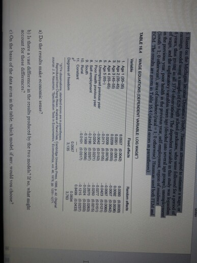
5. Based on the Michigan Income Dynamics Study, Hausman attempted to estimate a wags of canine modele s ple of 629 high school prad , who were followed for a paneda years, thus geving in all 3774 observations. The dependent variable in this study was logarithm of wage, and the explanatory vanables were ape (divided into several age groups), unemployment in the previous year, poor health in the previous year,self employment, region of residence (South = 1:0 otherwise) area of residence (rural = 1; 0 otherwise) Hamand both FEM and ECM The results are given in Table 16.4 (standard errors in parentheses TABLE 16.4 WAGE EQUATIONS (DEPENDENT VARIABLE: LOG WAGE" Variable Fixed effects Random fects 1. Ago 1 (20-35) 2. Ago 235-45) 3. Ago 45-55) 4. Ago 4 (55-65) 5. Age 5 (65) 6. Unemployed previous year 7. Poor health provious year 8. Self-employment 9. South 10. Mural 11. Constant 0.0567 10.00421 0.0351 0.0051) 0.0209 (0.0055) 0.0209 0.0078 0.017110.01561 -0.0012 00153] -0.0204 (00221) -0.210 10.0297) 0.1560 10.0666) -0.0101100017) 0,0390 0.0033) 0.0092 (0.0035) -0.0007 (0.0042) -0.0097 0.0060) -0.0423 (00121) -0.0077 (0.0151) -0.0250 10.0.2151 -0.2570 10.0263) -0.0024 (0.0333) -0.1215 (0.0237) 0.84.99 10.0433) Degree of freedom 374 observation Standard rore in parents Reproduced from Chang Hsiao. An o Pene Date Combedge University Press. p. 42. Ongina SOJ AHerman Specifications in finem contato 197 PO 1251-127 a) Do the results make economic sense? b) Is there a vast difference in the results produced by the two models? If so, what might account for these differences? c) On the basis of the data given in the table, which model, if any, would vou choose? 5. Based on the Michigan Income Dynamics Study, Hausman attempted to estimate a wags of canine modele s ple of 629 high school prad , who were followed for a paneda years, thus geving in all 3774 observations. The dependent variable in this study was logarithm of wage, and the explanatory vanables were ape (divided into several age groups), unemployment in the previous year, poor health in the previous year,self employment, region of residence (South = 1:0 otherwise) area of residence (rural = 1; 0 otherwise) Hamand both FEM and ECM The results are given in Table 16.4 (standard errors in parentheses TABLE 16.4 WAGE EQUATIONS (DEPENDENT VARIABLE: LOG WAGE" Variable Fixed effects Random fects 1. Ago 1 (20-35) 2. Ago 235-45) 3. Ago 45-55) 4. Ago 4 (55-65) 5. Age 5 (65) 6. Unemployed previous year 7. Poor health provious year 8. Self-employment 9. South 10. Mural 11. Constant 0.0567 10.00421 0.0351 0.0051) 0.0209 (0.0055) 0.0209 0.0078 0.017110.01561 -0.0012 00153] -0.0204 (00221) -0.210 10.0297) 0.1560 10.0666) -0.0101100017) 0,0390 0.0033) 0.0092 (0.0035) -0.0007 (0.0042) -0.0097 0.0060) -0.0423 (00121) -0.0077 (0.0151) -0.0250 10.0.2151 -0.2570 10.0263) -0.0024 (0.0333) -0.1215 (0.0237) 0.84.99 10.0433) Degree of freedom 374 observation Standard rore in parents Reproduced from Chang Hsiao. An o Pene Date Combedge University Press. p. 42. Ongina SOJ AHerman Specifications in finem contato 197 PO 1251-127 a) Do the results make economic sense? b) Is there a vast difference in the results produced by the two models? If so, what might account for these differences? c) On the basis of the data given in the table, which model, if any, would vou choose