Help solve with correct answers. TY!!

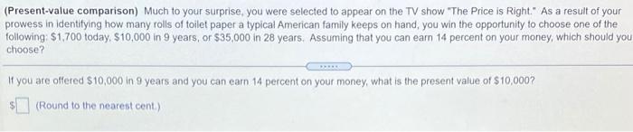
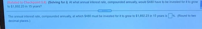
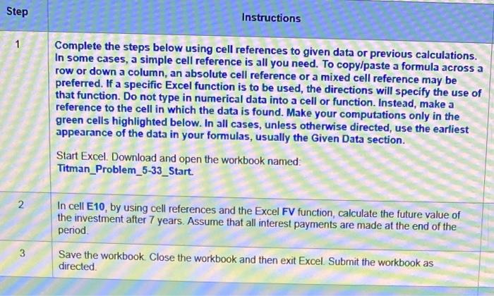
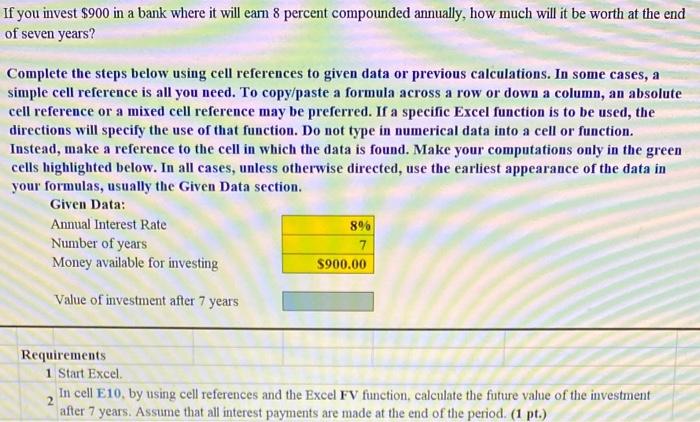
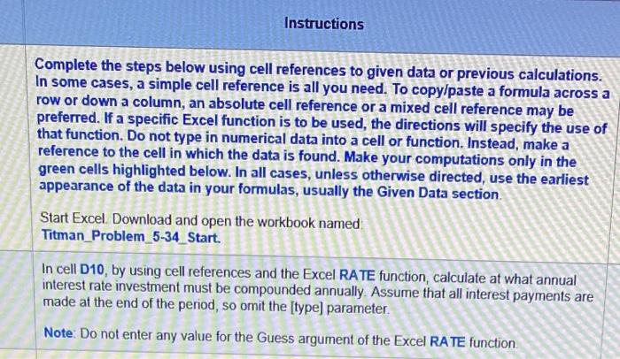
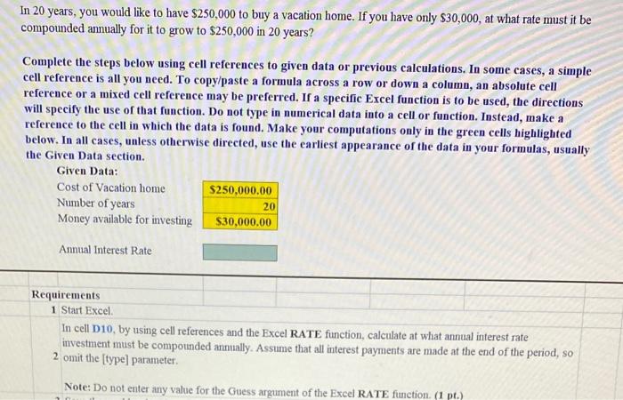
(Present-value comparison) Much to your surprise, you were selected to appear on the TV show "The Price is Right." As a result of your prowess in identifying how many rolls of toilet paper a typical American family keeps on hand, you win the opportunity to choose one of the following $1,700 today, $10,000 in 9 years, or $35,000 in 28 years. Assuming that you can earn 14 percent on your money, which should you choose? If you are offered $10,000 in 9 years and you can earn 14 percent on your money, what is the present value of $10,000? (Round to the nearest cent) (Related to Checkpoint 5.6) (Solving for 1) At what annual interest rate, compounded annually, would $480 have to be invested for it to grow to $1,892.23 in 15 years? The annual interest rate, compounded annually, at which $480 must be invested for it to grow to S1,892 23 in 15 years is % (Round to two decimal places.) Step Instructions 1 Complete the steps below using cell references to given data or previous calculations. In some cases, a simple cell reference is all you need. To copy/paste a formula across a row or down a column, an absolute cell reference or a mixed cell reference may be preferred. If a specific Excel function is to be used, the directions will specify the use of that function. Do not type in numerical data into a cell or function. Instead, make a reference to the cell in which the data is found. Make your computations only in the green cells highlighted below. In all cases, unless otherwise directed, use the earliest appearance of the data in your formulas, usually the Given Data section. Start Excel. Download and open the workbook named Titman_Problem_5-33_Start. N In cell E10, by using cell references and the Excel FV function, calculate the future value of the investment after 7 years. Assume that all interest payments are made at the end of the period 3 Save the workbook Close the workbook and then exit Excel Submit the workbook as directed If you invest $900 in a bank where it will eam 8 percent compounded annually, how much will it be worth at the end of seven years? Complete the steps below using cell references to given data or previous calculations. In some cases, a simple cell reference is all you need. To copy/paste a formula across a row or down a column, an absolute cell reference or a mixed cell reference may be preferred. If a specific Excel function is to be used, the directions will specify the use of that function. Do not type in numerical data into a cell or function. Instead, make a reference to the cell in which the data is found. Make your computations only in the green cells highlighted below. In all cases, unless otherwise directed, use the earliest appearance of the data in your formulas, usually the Given Data section. Given Data: Annual Interest Rate Number of years 7 Money available for investing $900.00 896 Value of investment after 7 years Requirements 1 Start Excel In cell E10. by using cell references and the Excel FV function, calculate the future value of the investment after 7 years. Assume that all interest payments are made at the end of the period. (1 pt.) 2 Instructions Complete the steps below using cell references to given data or previous calculations. In some cases, a simple cell reference is all you need. To copy/paste a formula across a row or down a column, an absolute cell reference or a mixed cell reference may be preferred. If a specific Excel function is to be used, the directions will specify the use of that function. Do not type in numerical data into a cell or function. Instead, make a reference to the cell in which the data is found. Make your computations only in the green cells highlighted below. In all cases, unless otherwise directed, use the earliest appearance of the data in your formulas, usually the Given Data section Start Excel. Download and open the workbook named Titman_Problem_5-34_Start. In cell D10, by using cell references and the Excel RATE function, calculate at what annual interest rate investment must be compounded annually. Assume that all interest payments are made at the end of the period, so omit the [type] parameter. Note: Do not enter any value for the Guess argument of the Excel RATE function In 20 years, you would like to have $250,000 to buy a vacation home. If you have only $30,000, at what rate must it be compounded annually for it to grow to $250,000 in 20 years? Complete the steps below using cell references to given data or previous calculations. In some cases, a simple cell reference is all you need. To copy/paste a formula across a row or down a column, an absolute cell reference or a mixed cell reference may be preferred. If a specific Excel function is to be used, the directions will specify the use of that function. Do not type in numerical data into a cell or function. Instead, make a reference to the cell in which the data is found. Make your computations only in the green cells highlighted below. In all cases, unless otherwise directed, use the earliest appearance of the data in your formulas, usually the Given Data section. Given Data: Cost of Vacation home $250,000.00 Number of years 20 Money available for investing $30,000.00 Annual Interest Rate Requirements 1 Start Excel In cell D10, by using cell references and the Excel RATE function, calculate at what annual interest rate investment must be compounded annually. Assume that all interest payments are made at the end of the period, so 2 omit the [type] parameter. Note: Do not enter any value for the Guess argument of the Excel RATE function. (1 pt.)