Question: Help! Thank you Summarize Data in a PivotTable and a PivotChart 1. Open BillingSummary4Q.xlsx and save it with the name 4-BillingSummary4Q. 2. Create a PivotTable

Help! Thank you

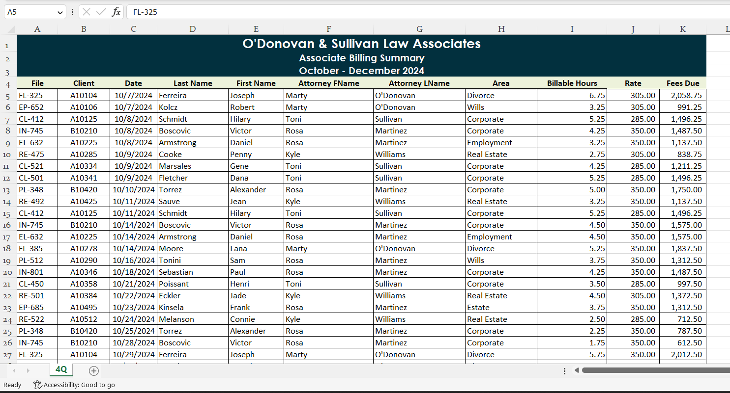
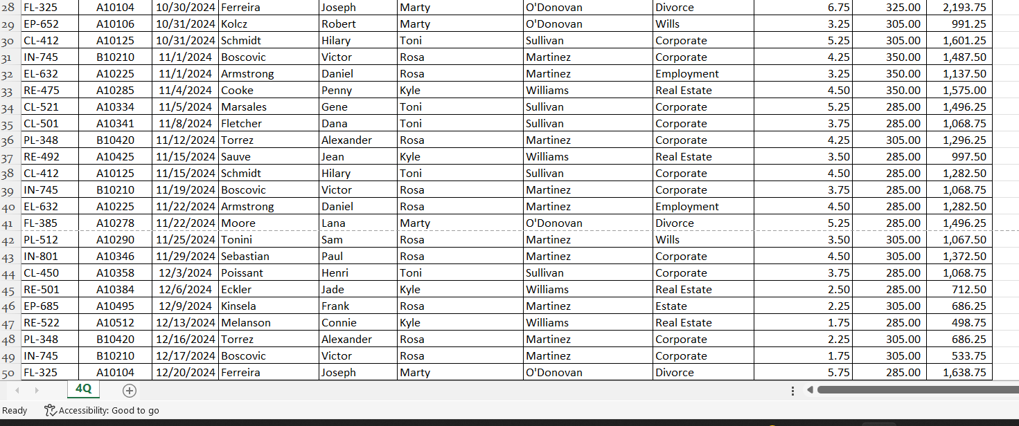
Summarize Data in a PivotTable and a PivotChart

1. Open BillingSummary4Q.xlsx and save it with the name 4-BillingSummary4Q.

2. Create a PivotTable in a new worksheet as follows:

a. Display the range named FourthQ and then insert a PivotTable in a new worksheet.

b. Add the Attorney LName field as rows.

c. Add the Area field as columns.

d. Sum the Fees Due field.

3. Apply the Light Blue, Pivot Style Medium 9 style (second column, second row in the Medium section) to the PivotTable.

4. Apply the Comma format with no digits after the decimal point to the values. Change the width of columns B through H to 13 characters. Remove the Autofit column widths on update check mark in the PivotTable Options dialog box. Right-align the Martinez, ODonovan, Sullivan, Williams, and Grand Total labels in column A.

5. Name the worksheet PivotTable and then do the following:

a. In cell A1, type Associate Billing Summary. Change the font to 14-point Arial and apply bold formatting. Merge and center the text across the PivotTable.

b. In cell A2, type October - December 2024. Change the font to 14-point Arial and apply bold formatting. Merge and center the text across the PivotTable.

c. Change the page layout to Landscape orientation and then preview the PivotTable.

6. Drill down cell H5. Autofit column C. Name the worksheet Martinez.

7. Create a PivotChart from the PivotTable using the 3D Stacked Column chart type and move the chart to its own sheet named PivotChart.

8. Apply Style 7 (seventh style in the Chart Styles gallery) to the PivotChart.

9. Filter the PivotChart by the attorney name Martinez.

10. Preview the PivotChart.

11. Save and then close 4-BillingSummary4Q.xlsx.

Filter a PivotTable Using a Slicer and a Timeline

1. Open 4-BillingSummary4Q.xlsx and save it with the name 4-BillingSummary4Q-5.

2. Click the PivotTable sheet to view the PivotTable.

3. Remove the filter to display all the attorney names.

4. Insert a Slicer pane for the Area field and move the Slicer pane below the PivotTable. Make the height of the Slicer pane 2.2 inches.

5. Using the Slicer pane, filter the PivotTable by the Corporate field. Add the Divorce option.

6. Insert a Timeline pane for the Date field and move the Timeline pane right of the Slicer pane.

7. Using the Timeline pane, filter the PivotTable for October to November 2024.

8. Save and then close 4-BillingSummary4Q-5.xlsx.

Help! Thank you Summarize Data in a PivotTable and a PivotChart 1.

Open BillingSummary4Q.xlsx and save it with the name 4-BillingSummary4Q. 2. Create a

Step by Step Solution

There are 3 Steps involved in it

1 Expert Approved Answer

Step: 1 Unlock blur-text-image

Question Has Been Solved by an Expert!

Get step-by-step solutions from verified subject matter experts

Step: 2 Unlock

Step: 3 Unlock

Students Have Also Explored These Related Databases Questions!

Assessment 4 Summarize Data in a PivotTable and a PivotChart Open BillingSummary 4 Q . xlsx and save it with the name 4 - BillingSummary 4 Q . Create a PivotTable in a new worksheet as follows: a ....

Apply Your Skills EA4-A1 Edit an Inventory Listing and Create a PivotTable for Educational Endeavors In this exercise , you will compile summary data based on an inventory listing for Educational...

How do I upload the Microsoft excel in chegg there wasn't any option. EA4-A2 Edit an Inventory Listing and Create a PivotTable for Electronic Worl Then you will determine the inventory balance for a...

EA4-A2 Edit an Inventory Listing and Create a PivotTable for Electronic World In this exercise, you will compile summary data based on an inventory listing for Electronic World. Then you will...

Apply Your Skills EA4-A1 Edit an Inventory Listing and Create a PivotTable for Educational Endeavors In this exercise, you will compile summary data based on an inventory listing for Educational...

Then you will determine the inventory balance for a product category using three methods. Last, you will create a PivotTable and a PivotChart. 1. Open EA4-A2-Inventory from your Chapter 04 folder and...

WEEK # 1 - EXERCISES Exercise 1 You oversee a young and growing business. You have identified the various factors (sources of revenue and expenses) that influence the business as shown in the table...

compile summary data based on an inventory listing for Electronic World. Then you will determine the inventory balance for a product category using three methods. Last, PivotTable and a PivotChart....

What is colloid? Write down the properties of colloids.

During the onset of the global financial crisis, many of the world's central banks and governments prevented large banks from failing. If these institutions had allowed this to occur, there would...

Which of the following statements describes a liquidity premium? Group of answer choices It is a premium added by investors to the real risk - free rate of return to account for inflation that is...

Flower, who has an at-risk basis in a partnership of $75,000, receives a nonliquidating distribution property (fair market value $58,000, adjusted basis to the partnership $40,000) and $10,000 cash....

2. The Big Brothers/Big Sisters of America is the oldest teen mentor organization in the country. Go to its Web site at www.bbbsa.org. Read about the corporate partners; read the newsletters and...

7. The Department of Labors Occupational Information Network (O*NET) is designed to meet the goal of promoting the education, training, counseling, and employment needs of the American work force. Go...

9. What are some potential advantages and disadvantages of attitude-awareness-based diversity training programs?