help with formulas in step 8 and step 13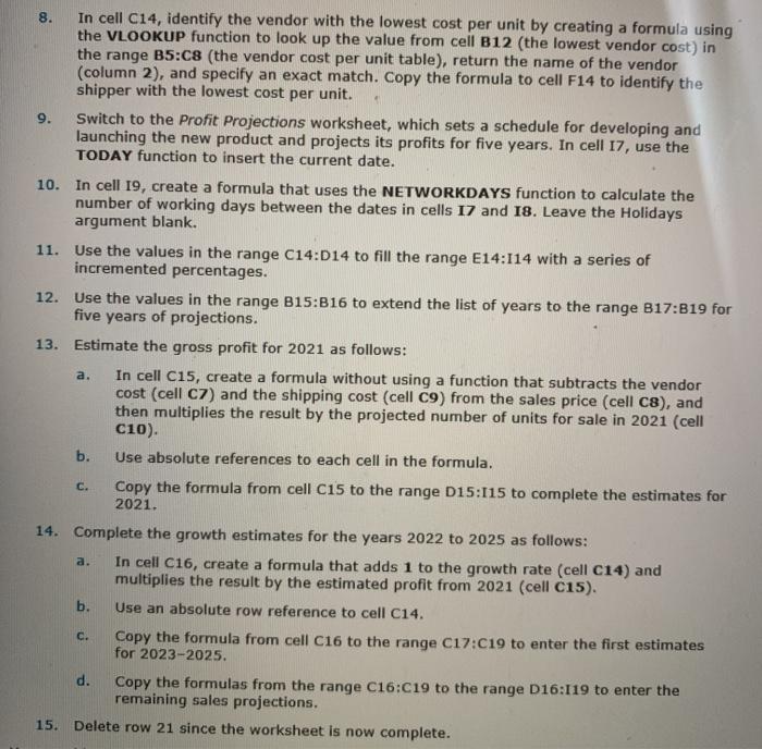

also step 10

8. In cell C14, identify the vendor with the lowest cost per unit by creating a formula using the VLOOKUP function to look up the value from cell B12 (the lowest vendor cost) in the range B5:C8 (the vendor cost per unit table), return the name of the vendor (column 2), and specify an exact match. Copy the formula to cell F14 to identify the shipper with the lowest cost per unit. Switch to the Profit Projections worksheet, which sets a schedule for developing and launching the new product and projects its profits for five years. In cell 17, use the TODAY function to insert the current date. 10. In cell 19, create a formula that uses the NETWORKDAYS function to calculate the number of working days between the dates in cells 17 and 18. Leave the Holidays argument blank. 11. Use the values in the range C14:014 to fill the range E14:114 with a series of incremented percentages. 12. Use the values in the range B15:B16 to extend the list of years to the range B17:319 for five years of projections. 13. Estimate the gross profit for 2021 as follows: In cell C15, create a formula without using a function that subtracts the vendor cost (cell c7) and the shipping cost (cell c9) from the sales price (cell C8), and then multiplies the result by the projected number of units for sale in 2021 (cell C10). b. Use absolute references to each cell in the formula. Copy the formula from cell C15 to the range D15:115 to complete the estimates for 2021. 14. Complete the growth estimates for the years 2022 to 2025 as follows: a. In cell C16, create a formula that adds 1 to the growth rate (cell C14) and multiplies the result by the estimated profit from 2021 (cell c15). b. Use an absolute row reference to cell C14. Copy the formula from cell C16 to the range C17:019 to enter the first estimates for 2023-2025. d. Copy the formulas from the range C16:C19 to the range D16:119 to enter the remaining sales projections. Delete row 21 since the worksheet is now complete. a. C. c. 15. 8. In cell C14, identify the vendor with the lowest cost per unit by creating a formula using the VLOOKUP function to look up the value from cell B12 (the lowest vendor cost) in the range B5:C8 (the vendor cost per unit table), return the name of the vendor (column 2), and specify an exact match. Copy the formula to cell F14 to identify the shipper with the lowest cost per unit. Switch to the Profit Projections worksheet, which sets a schedule for developing and launching the new product and projects its profits for five years. In cell 17, use the TODAY function to insert the current date. 10. In cell 19, create a formula that uses the NETWORKDAYS function to calculate the number of working days between the dates in cells 17 and 18. Leave the Holidays argument blank. 11. Use the values in the range C14:014 to fill the range E14:114 with a series of incremented percentages. 12. Use the values in the range B15:B16 to extend the list of years to the range B17:319 for five years of projections. 13. Estimate the gross profit for 2021 as follows: In cell C15, create a formula without using a function that subtracts the vendor cost (cell c7) and the shipping cost (cell c9) from the sales price (cell C8), and then multiplies the result by the projected number of units for sale in 2021 (cell C10). b. Use absolute references to each cell in the formula. Copy the formula from cell C15 to the range D15:115 to complete the estimates for 2021. 14. Complete the growth estimates for the years 2022 to 2025 as follows: a. In cell C16, create a formula that adds 1 to the growth rate (cell C14) and multiplies the result by the estimated profit from 2021 (cell c15). b. Use an absolute row reference to cell C14. Copy the formula from cell C16 to the range C17:019 to enter the first estimates for 2023-2025. d. Copy the formulas from the range C16:C19 to the range D16:119 to enter the remaining sales projections. Delete row 21 since the worksheet is now complete. a. C. c. 15