Here is the data that came before the question and one needed for it

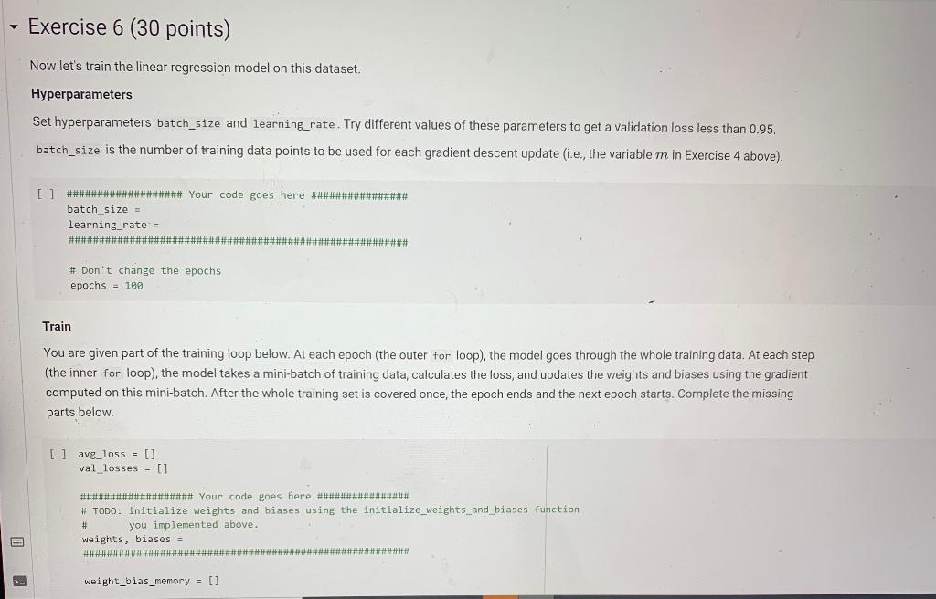
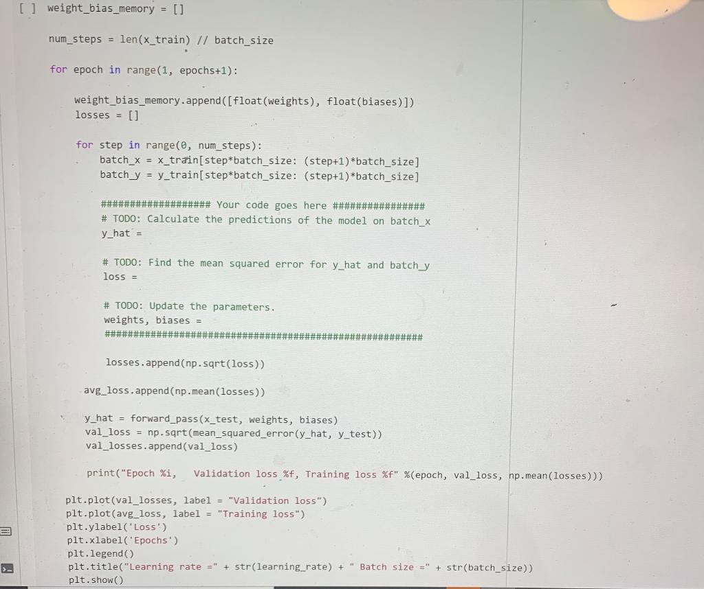
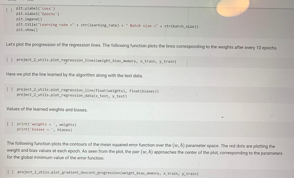
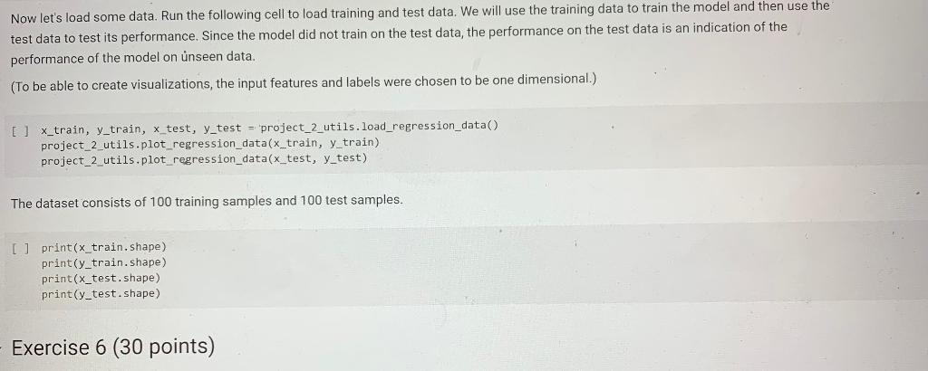
Now let's load some data. Run the following cell to load training and test data. We will use the training data to train the model and then use the test data to test its performance. Since the model did not train on the test data, the performance on the test data is an indication of the performance of the model on unseen data. (To be able to create visualizations, the input features and labels were chosen to be one dimensional.) [x_train, y_train, x_test, y_test = 'project_2_utils. load_regression_data() project_2_utils.plot_regression_data(x_train, y_train) project_2_utils.plot_regression_data(x_test, y_test) The dataset consists of 100 training samples and 100 test samples. Il print(x_train.shape) print(y_train.shape) print(x_test.shape) print(y_test.shape) Exercise 6 (30 points) Exercise 6 (30 points) Now let's train the linear regression model on this dataset. Hyperparameters Set hyperparameters batch_size and learning_rate. Try different values of these parameters to get a validation loss less than 0.95. batch_size is the number of training data points to be used for each gradient descent update (i.e., the variable m in Exercise 4 above). [] ################### Your code goes here ################ batch_size = learning_rate= ######################################*****#*############# # Don't change the epochs epochs = 100 Train You are given part of the training loop below. At each epoch (the outer for loop), the model goes through the whole training data. At each step (the inner for loop), the model takes a mini-batch of training data, calculates the loss, and updates the weights and biases using the gradient computed on this mini-batch. After the whole training set is covered once, the epoch ends and the next epoch starts. Complete the missing parts below. [ ] avg_loss = [] val_losses = [] ################### Your code goes here ################ # TODO: Initialize weights and biases using the initialize_weights_and_biases function you implemented above. weights, biases = ################# ######## # weight_bias_memory = [] weight_bias_memory = [] num_steps = len(x_train) // batch_size for epoch in range(1, epochs+1): weight_bias_memory.append([float(weights), float(biases)]) losses = [] for step in range(0, num_steps): batch_x = x_train(step*batch_size: (step+1)*batch_size] batch y = y_train(step*batch_size: (step+1)*batch_size] ################### Your code goes here ################ # TODO: Calculate the predictions of the model on batch_x y_hat = # TODO: Find the mean squared error for y_hat and batchy loss = # TODO: Update the parameters. weights, biases = losses.append(np.sqrt(loss)) avg_loss.append(np.mean(losses)) y_hat = forward_pass (x_test, weights, biases) val_loss = np.sqrt(mean_squared_error(y_hat, y_test)) val_losses.append(val_loss) print("Epoch %i, Validation loss %f, Training loss %f" %(epoch, val_loss, np.mean(losses))) EB plt.plot(val_losses, label = "Validation loss") plt.plot(avg_loss, label = "Training loss") plt.ylabel('Loss') plt.xlabel('Epochs) plt.legend plt.title("Learning rate =" + str(learning_rate) + " Batch size=" plt.show() + str(batch_size)) [] plt.ylabel('Loss') plt.xlabel('Epochs') plt.legend plt.title("Learning rate =" + str(learning_rate) + " Batch size =" + str(batch_size)) plt.show() Let's plot the progression of the regression lines. The following function plots the lines corresponding to the weights after every 10 epochs. [ ] project_2_utils.plot_regression_lines (weight_bias_memory, x_train, y_train) Here we plot the line learned by the algorithm along with the test data. [] project_2_utils.plot_regression_line (float(weights), float(biases)) project_2_utils.plot_regression_data(x_test, y_test) Values of the learned weights and biases. [] print('weights = ', weights) print('biases = ', biases) The following function plots the contours of the mean squared error function over the w, b) parameter space. The red dots are plotting the weight and bias values at each epoch. As seen from the plot, the pair (w,b) approaches the center of the plot, corresponding to the parameters for the global minimum value of the error function. [] project_2_utils.plot_gradient_descent_progression (weight_bias_memory, x_train, y_train) Now let's load some data. Run the following cell to load training and test data. We will use the training data to train the model and then use the test data to test its performance. Since the model did not train on the test data, the performance on the test data is an indication of the performance of the model on unseen data. (To be able to create visualizations, the input features and labels were chosen to be one dimensional.) [x_train, y_train, x_test, y_test = 'project_2_utils. load_regression_data() project_2_utils.plot_regression_data(x_train, y_train) project_2_utils.plot_regression_data(x_test, y_test) The dataset consists of 100 training samples and 100 test samples. Il print(x_train.shape) print(y_train.shape) print(x_test.shape) print(y_test.shape) Exercise 6 (30 points) Exercise 6 (30 points) Now let's train the linear regression model on this dataset. Hyperparameters Set hyperparameters batch_size and learning_rate. Try different values of these parameters to get a validation loss less than 0.95. batch_size is the number of training data points to be used for each gradient descent update (i.e., the variable m in Exercise 4 above). [] ################### Your code goes here ################ batch_size = learning_rate= ######################################*****#*############# # Don't change the epochs epochs = 100 Train You are given part of the training loop below. At each epoch (the outer for loop), the model goes through the whole training data. At each step (the inner for loop), the model takes a mini-batch of training data, calculates the loss, and updates the weights and biases using the gradient computed on this mini-batch. After the whole training set is covered once, the epoch ends and the next epoch starts. Complete the missing parts below. [ ] avg_loss = [] val_losses = [] ################### Your code goes here ################ # TODO: Initialize weights and biases using the initialize_weights_and_biases function you implemented above. weights, biases = ################# ######## # weight_bias_memory = [] weight_bias_memory = [] num_steps = len(x_train) // batch_size for epoch in range(1, epochs+1): weight_bias_memory.append([float(weights), float(biases)]) losses = [] for step in range(0, num_steps): batch_x = x_train(step*batch_size: (step+1)*batch_size] batch y = y_train(step*batch_size: (step+1)*batch_size] ################### Your code goes here ################ # TODO: Calculate the predictions of the model on batch_x y_hat = # TODO: Find the mean squared error for y_hat and batchy loss = # TODO: Update the parameters. weights, biases = losses.append(np.sqrt(loss)) avg_loss.append(np.mean(losses)) y_hat = forward_pass (x_test, weights, biases) val_loss = np.sqrt(mean_squared_error(y_hat, y_test)) val_losses.append(val_loss) print("Epoch %i, Validation loss %f, Training loss %f" %(epoch, val_loss, np.mean(losses))) EB plt.plot(val_losses, label = "Validation loss") plt.plot(avg_loss, label = "Training loss") plt.ylabel('Loss') plt.xlabel('Epochs) plt.legend plt.title("Learning rate =" + str(learning_rate) + " Batch size=" plt.show() + str(batch_size)) [] plt.ylabel('Loss') plt.xlabel('Epochs') plt.legend plt.title("Learning rate =" + str(learning_rate) + " Batch size =" + str(batch_size)) plt.show() Let's plot the progression of the regression lines. The following function plots the lines corresponding to the weights after every 10 epochs. [ ] project_2_utils.plot_regression_lines (weight_bias_memory, x_train, y_train) Here we plot the line learned by the algorithm along with the test data. [] project_2_utils.plot_regression_line (float(weights), float(biases)) project_2_utils.plot_regression_data(x_test, y_test) Values of the learned weights and biases. [] print('weights = ', weights) print('biases = ', biases) The following function plots the contours of the mean squared error function over the w, b) parameter space. The red dots are plotting the weight and bias values at each epoch. As seen from the plot, the pair (w,b) approaches the center of the plot, corresponding to the parameters for the global minimum value of the error function. [] project_2_utils.plot_gradient_descent_progression (weight_bias_memory, x_train, y_train)