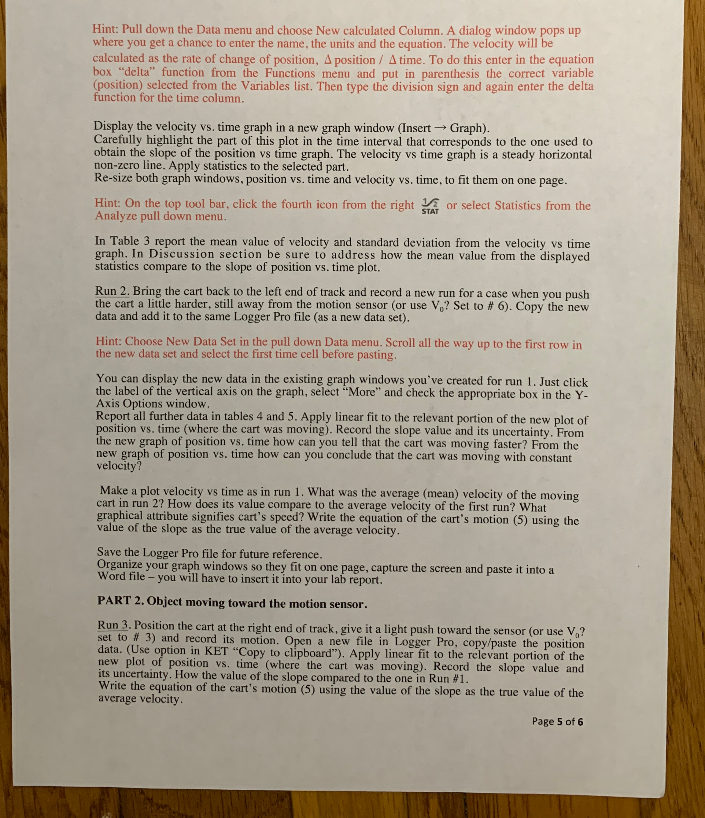
Hint: Pull down the Data menu and choose New calculated Column. A dialog window pops up where you get a chance to enter the name, the units and the equation. The velocity will be calculated as the rate of change of position, $$ position $/$ time. To do this enter in the equation box "delta" function from the Functions menu and put in parenthesis the correct variable $($position$)$ selected from the Variables list. Then type the division sign and again enter the delta function for the time column.

Display the velocity vs$.$ time graph in a new graph window $($Insert $$ Graph$).$

Carefully highlight the part of this plot in the time interval that corresponds to the one used to obtain the slope of the position vs time graph. The velocity vs time graph is a steady horizontal non$-$zero line. Apply statistics to the selected part.

Re$-$size both graph windows, position vs$.$ time and velocity vs$.$ time, to fit them on one page.

Hint: On the top tool bar, click the fourth icon from the right $\frac{1}{\text{s}\text{t}\text{a}\text{T}}$ or select Statistics from the Analyze pull down menu.

In Table $3$ report the mean value of velocity and standard deviation from the velocity vs time graph. In Discussion section be sure to address how the mean value from the displayed statistics compare to the slope of position vs$.$ time plot.

Run $2.$ Bring the cart back to the left end of track and record a new run for a case when you push the cart a little harder, still away from the motion sensor $($or use $V_0?$ Set to # $6).$ Copy the new data and add it to the same Logger Pro file $($as a new data set$).$

Hint: Choose New Data Set in the pull down Data menu. Scroll all the way up to the first row in the new data set and select the first time cell before pasting.

You can display the new data in the existing graph windows you've created for run $1.$ Just click the label of the vertical axis on the graph, select "More" and check the appropriate box in the YAxis Options window.

Report all further data in tables $4$ and $5.$ Apply linear fit to the relevant portion of the new plot of position vs$.$ time $($where the cart was moving$).$ Record the slope value and its uncertainty. From the new graph of position vs$.$ time how can you tell that the cart was moving faster? From the new graph of position vs$.$ time how can you conclude that the cart was moving with constant velocity?

Make a plot velocity vs time as in run $1.$ What was the average $($mean$)$ velocity of the moving cart in run $2?$ How does its value compare to the average velocity of the first run? What graphical attribute signifies cart's speed? Write the equation of the cart's motion $(5)$ using the value of the slope as the true value of the average velocity.

Save the Logger Pro file for future reference.

Organize your graph windows so they fit on one page, capture the screen and paste it into a Word file $-$ you will have to insert it into your lab report.

PART $2.$ Object moving toward the motion sensor$.$

Run $3.$ Position the cart at the right end of track, give it a light push toward the sensor $($or use $V_0?$ set to # $3)$ and record its motion. Open a new file in Logger Pro, copy$/$paste the position data. $($Use option in KET "Copy to clipboard"$).$ Apply linear fit to the relevant portion of the new plot of position vs$.$ time $($where the cart was moving$).$ Record the slope value and its uncertainty. How the value of the slope compared to the one in Run #$1.$

Write the equation of the cart's motion $(5)$ using the value of the slope as the true value of the average velocity.

Page $5$ of $6$