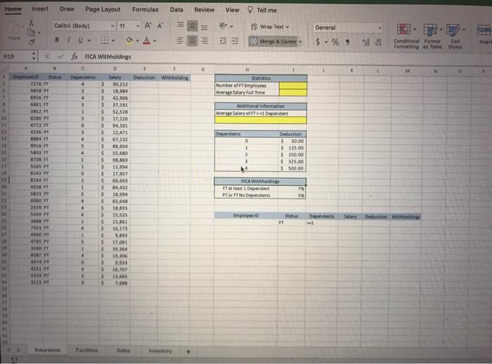
Home Insert Draw Page Layout Formulas Data Review View Tell me Calibel (Body 11 ' ' Wrap Text General BIU Merge Center $ % 9 *all-23 Call Conditional Format Formatting Table H19 H M N 0 4 Statistics Number of Ft Employees Averaro Salary Time T 0 10 Impree ID Status 7276 FT 55 P 1936 FT 6881 FT 1852 FT GSRO PT 4772 FT 4206 BB FT 1916 FT Additional information Average Salary of T> Dependent 12 Dependents 14 0 1 2 Deduction 5 50.00 $ 125.00 $ 25000 $325.00 $ 500.00 16 fx RICA Withholdings D Det Deduction withholding 4 $ 90 212 2 $ 11,954 4 $ 42,905 5 5 37.191 1 5 52,520 5 $ 17,126 0 5 94,101 $ 12.471 4 $ 67,132 $ 88.604 $ 55.680 1 $ 9.86 1 $ 11.994 0 $ 17.257 2 $ 66.63 1 5 54.432 S 5 16.994 $ 65.648 & $ 16835 . 5 15,525 1 $ 35.161 4 5 16.173 1 $ 9,893 5 5 17,081 1 $ 33,364 4 5 10,300 0 9,033 $ 16,707 5 13.665 0 5 8700 FT 5565 FT IR B16 T 10 21 22 FICA WItholdings FT 1 Depec PT O FT No Dependent SX 24 Employee 10 Status FT Dependent Deduction withbolding 5839 PT GOLO FT 2550 FT 556 Ft 34 PT 7351 FT 49 PT 4785 FT 1000 FT 2007 474 FT 4251 FT 12 PT 3123 1 31 10 Inson Farabus inventory + Hint: - Function copied down column F Data in column F formatted with Accounting Number format Apply conditional formatting to the range C5-C34 that highlights any dependents that are greater than 3 with Light Red Fill and Dark Red Text, In the Styles group, click Conditional Formatting Conditional formatting applied to range C5C34 -Dependents greater than 3 highlighted -Light Red Fill Dark Red Text 9 Click cell H10, and enter an AVERAGEIFS function to determine the average 3 salary of full-time employees with at least one dependent. Format the results in Accounting Number Format Hint AVERAGEIFS (average-range. criteria-rangel criteria.) - AVERAGEIFS function used correctly -Returns average salary of full-time employees with at least one dependent - Result formatted with Accounting number format 10 Use Advanced Filtering to restrict the data to only display full-time employees 2 with at least one dependent. Place the results in cell A37. Use the criteria in the range H24 M25 to complete the function Hint: On the Data tab, in the Sort & Filter group, click Advanced -Advance filtering used correctly -Criteria in range H24 M25 used to complete function -Results placed in cell A37 11 Ensure that the Facilities worksheet is active. Use Goal Seek to reduce the monthly payment in cell B6 to the optimal value of $6000. Complete this task by changing the Loan amount in cell E6. Hint: On the Datatab, in the Forecast group, click What If Analysis, Goal seek used properly Monthly payment is reduced to 56000 -Loan amount in cell E6 changed correctly 12 Create the following three scenarios using Scenario Manager. The scenarios s should change the cells B2, B8, and E6. Good B7,0325 B85 E6275000 Most Likely B7.057 BS-5 E6312227.32 Bad B7-0700 B8-3 E6 - 350000 Create a Scenario Summary Report based on the value in cell B6. Format the new report appropriately Hint. On the Data tab, in the Forecast group, click What If Analysis. Scenario Manager --Three scenarios created with Correct name -Correct values Summary Report is based on the value in cell B6 New report formatted appropriately 13 Ensure that the Facilities worksheet is active Enter a reference to the beginning 4 loan balance in cell B12 and enter a reference to the payment amount in cell C12 Hint: -Facilities worksheet is active -Reference to beginning loan balance in cell B12 im Call CM Date 3 14 Enter a function in cell D12, based on the payment and lon detail that calculates the amount of interest paid on the first payment. Be sure to use the appropriate absolute relative, or mixed cell references The function is IPMT frate per per-py.IM.ltpell Correct cell referenced in the IPMT functies to calculate the amount of interest paid en first payment Appropriate cell referencing (absolute cell reference, and relative cell reference must be used in their places to get the complete marks here) Function in D12 return correct value 15 Enter a function in cell E12, based on the payment and loan details, that calculates the amount of principal paid on the first payment. Be sure to use the appropriate absolute relative of mixed cell references The function is - PPT rate.peraper -p M.type Correet cell referenced in the PPMT function to calculate the amount of principal paid on first payment - Appropriate cell referencing (blue cell reference, and relative cell reference must be used in their places to get the complete marks here) -Function in B12 rotum correct value 16 Enter a formula in cell F12 to calculate the remaining balance after the current 2 payment. The remaining balance is calculated by subtracting the principal payment from the balance in column Hint: - Formula in cell F12 used correct cells Displayed correct result 17 Entet function in cell G12, based on the payment and loan details, that calculates the amount of cumulative interest paid on the first payment. Be sure to use the appropriate absolute, relative, or mixed cell references The function is-CUMIPM Terate, nper.px, start period, end period. type Correct cell referenced in the CUMIPMT function to calculate the amount of Cumulative interest paid co the first payment Appropriate cell referencing (absolute cell reference, and relative cell reference must be used in their places to get the complete marks here) Function in G12 retum correct value 18 Enter a function in cell 12, based on the payment and loan details, that 3 calculates the amount of cumulative principal paid on the first payment. Be sure to use the appropriate absolute, relative or mixed cell references Hint The function is --CUMPRINCrate, per, prestart period, end period type) Correct cell referenced in the CUMPRINC function to calculate the amount of cumulative principal paid on the first payment - Appropriate cell referencing (absolute cell reference, and relative cell reference must be used in their places to get the complete marks here) Function in H12 retum correct value 19 Enter a reference to the remaining balance of payment in cell B13. Use the fill 3 handle to copy the functions created in the prior steps down to complete the amortization table Hint: -Value in B13 is a cell reference to Remaining Balance of Payment 1 (That is 13 cell reference F12 -Fill handle used to copy the above functions (functions created in Sep 13 to slept 19 down to complete amortization table 20 Ensure the Sales worksheet is active. Enter a function in cell B to create a 7 cudom transaction number. The transaction number should be comprised of the item number listed in cell C combined with the quantity in cell D and the first initial of the payment type in cell Ex. Use Auto Fill to copy the function deron completing the data in column Hint The function is C&DEXLEFTESI Sales Worksheet active - Function created in B Function returns -item number listed in cell CK combined with the quantity in cells and the first initial of the payment type in cell EN -Auto Fill used to copy the above function down to complete in column B 21 Entet a nested function in cells that displays the word Flag of the Payment 7 Type is Credit and the Amount is greater than or equal to 1000. Otherwise, the function will display a blank cell. Use Auto Fill to copy the functie down completing the data in column The function is IF (AND (logical Ilogical 2...) For example: IF (AND (ES-"Credit", logic 2."Flag"."> Nested function in cell G8 has correct criteria - Amount is greater than or equal to 54000 -Nested function in cell GR, displays a blank cell for other conditions - Auto Fill used to copy the above function down to complete in column 22 Create a data validation list in cells that displays Quantity, Payment Type 5 and Amount Hint: On the Data tab, in the Duta Tools group, click Data Validation. Allow. List Data list created in cells -List has Quantity. Payment Type, and Amount 23 Type the Trans 30038C in cells and electrontity from the validatie is 2 in cell DS Hint: -Transit 30038C in cell BS - Validation List Quantity displayed in cell DS 24 Enter a nessed lookup function in cells that evaluates the Trans #icell B5 as 3 well as the Category in cell Ds, and returns the results based on the data in the range AB:F32 Hint: Use function INDEXO) and MATCH). -Nested lookup function in cell FS -Evaluates Trans in cell BS. Category in cell DS -Returns results based on dute in range AX:F32 25 Create a Pivot Table based on the range A7:632. Place the Prvee Table in cell 175 on the current worksheet. Mace Payment Type in the Rews box and Amount in the Values box, Format the Amount with Accounting Number Format Hint: On the Insert tab, in the Tables group, select Pivot Table Range A.G2 used to create Pivot Table Pivot Table placed in cell 117 in current worksheet -Payment Type in the Rows box area Amount in the Values box arca Amount formatted with Accounting Format 26 Insert a PivoChart using the Pie chart type based on the data. Place the upper + letcome of the chart inside cell 122. Format he Legend of the chart to appear at the bottom of the chur arca. Format the Data Labels to appear on the Outiede end of the chart Note. Ma usets, select the range 118220, on the Insert tab, click Recommended Charts, and then click Pie Format the legend, and apply the data labels as specified Hint: On the Analyze tab, in the Tools group, click PivoChart -Create PivotChart Pie Chart based on above data -Upper left comer of the PivotChart Pie Chart placed in cell 122 Legend of PivotChart formatted to appear at the bottom of Chartara Data Labels to appear on the Outside end of the chart 27 Insert a Slicer based on Dute. Place the upper-left comer of the Slicer inside cell 3 Hint On the Insert tab, in the Filters group, and click Slicer Slicer based on Date from Pivot Table -Upper-left corner of the Slicer in cell LX Slicer has right values 28 Ensure the Inventory worksheet is active. Import the Access database App Cap Inventory.ch into the worksheet starting in cell A3 Note, Mac users, download and import the delimited Inventory.file into the worksheet starting in cell A3. Hint Use the tools on the Duta tab to import the file as specified On the Data tab, in the Get & Transform Data group, click Get Duta. From Database, From Microsoft Access database. Load -Database file imported to Inventory worksheet -Table starts from cell A3 -Table has right heading and data 29 Create a footer with your name on the left the shoe code in the center and the 2 file name on the right for each worksheet Hint: For each worksheet: Name on left side of footer Sheet code in the Center -File same on the right side 30 Save and close the file Submit ACC2343 Final Manufacturing Las Finster Total Point 100 Home Insert Draw Page Layout Formulas Data Review View Tell me Calibel (Body 11 ' ' Wrap Text General BIU Merge Center $ % 9 *all-23 Call Conditional Format Formatting Table H19 H M N 0 4 Statistics Number of Ft Employees Averaro Salary Time T 0 10 Impree ID Status 7276 FT 55 P 1936 FT 6881 FT 1852 FT GSRO PT 4772 FT 4206 BB FT 1916 FT Additional information Average Salary of T> Dependent 12 Dependents 14 0 1 2 Deduction 5 50.00 $ 125.00 $ 25000 $325.00 $ 500.00 16 fx RICA Withholdings D Det Deduction withholding 4 $ 90 212 2 $ 11,954 4 $ 42,905 5 5 37.191 1 5 52,520 5 $ 17,126 0 5 94,101 $ 12.471 4 $ 67,132 $ 88.604 $ 55.680 1 $ 9.86 1 $ 11.994 0 $ 17.257 2 $ 66.63 1 5 54.432 S 5 16.994 $ 65.648 & $ 16835 . 5 15,525 1 $ 35.161 4 5 16.173 1 $ 9,893 5 5 17,081 1 $ 33,364 4 5 10,300 0 9,033 $ 16,707 5 13.665 0 5 8700 FT 5565 FT IR B16 T 10 21 22 FICA WItholdings FT 1 Depec PT O FT No Dependent SX 24 Employee 10 Status FT Dependent Deduction withbolding 5839 PT GOLO FT 2550 FT 556 Ft 34 PT 7351 FT 49 PT 4785 FT 1000 FT 2007 474 FT 4251 FT 12 PT 3123 1 31 10 Inson Farabus inventory + Hint: - Function copied down column F Data in column F formatted with Accounting Number format Apply conditional formatting to the range C5-C34 that highlights any dependents that are greater than 3 with Light Red Fill and Dark Red Text, In the Styles group, click Conditional Formatting Conditional formatting applied to range C5C34 -Dependents greater than 3 highlighted -Light Red Fill Dark Red Text 9 Click cell H10, and enter an AVERAGEIFS function to determine the average 3 salary of full-time employees with at least one dependent. Format the results in Accounting Number Format Hint AVERAGEIFS (average-range. criteria-rangel criteria.) - AVERAGEIFS function used correctly -Returns average salary of full-time employees with at least one dependent - Result formatted with Accounting number format 10 Use Advanced Filtering to restrict the data to only display full-time employees 2 with at least one dependent. Place the results in cell A37. Use the criteria in the range H24 M25 to complete the function Hint: On the Data tab, in the Sort & Filter group, click Advanced -Advance filtering used correctly -Criteria in range H24 M25 used to complete function -Results placed in cell A37 11 Ensure that the Facilities worksheet is active. Use Goal Seek to reduce the monthly payment in cell B6 to the optimal value of $6000. Complete this task by changing the Loan amount in cell E6. Hint: On the Datatab, in the Forecast group, click What If Analysis, Goal seek used properly Monthly payment is reduced to 56000 -Loan amount in cell E6 changed correctly 12 Create the following three scenarios using Scenario Manager. The scenarios s should change the cells B2, B8, and E6. Good B7,0325 B85 E6275000 Most Likely B7.057 BS-5 E6312227.32 Bad B7-0700 B8-3 E6 - 350000 Create a Scenario Summary Report based on the value in cell B6. Format the new report appropriately Hint. On the Data tab, in the Forecast group, click What If Analysis. Scenario Manager --Three scenarios created with Correct name -Correct values Summary Report is based on the value in cell B6 New report formatted appropriately 13 Ensure that the Facilities worksheet is active Enter a reference to the beginning 4 loan balance in cell B12 and enter a reference to the payment amount in cell C12 Hint: -Facilities worksheet is active -Reference to beginning loan balance in cell B12 im Call CM Date 3 14 Enter a function in cell D12, based on the payment and lon detail that calculates the amount of interest paid on the first payment. Be sure to use the appropriate absolute relative, or mixed cell references The function is IPMT frate per per-py.IM.ltpell Correct cell referenced in the IPMT functies to calculate the amount of interest paid en first payment Appropriate cell referencing (absolute cell reference, and relative cell reference must be used in their places to get the complete marks here) Function in D12 return correct value 15 Enter a function in cell E12, based on the payment and loan details, that calculates the amount of principal paid on the first payment. Be sure to use the appropriate absolute relative of mixed cell references The function is - PPT rate.peraper -p M.type Correet cell referenced in the PPMT function to calculate the amount of principal paid on first payment - Appropriate cell referencing (blue cell reference, and relative cell reference must be used in their places to get the complete marks here) -Function in B12 rotum correct value 16 Enter a formula in cell F12 to calculate the remaining balance after the current 2 payment. The remaining balance is calculated by subtracting the principal payment from the balance in column Hint: - Formula in cell F12 used correct cells Displayed correct result 17 Entet function in cell G12, based on the payment and loan details, that calculates the amount of cumulative interest paid on the first payment. Be sure to use the appropriate absolute, relative, or mixed cell references The function is-CUMIPM Terate, nper.px, start period, end period. type Correct cell referenced in the CUMIPMT function to calculate the amount of Cumulative interest paid co the first payment Appropriate cell referencing (absolute cell reference, and relative cell reference must be used in their places to get the complete marks here) Function in G12 retum correct value 18 Enter a function in cell 12, based on the payment and loan details, that 3 calculates the amount of cumulative principal paid on the first payment. Be sure to use the appropriate absolute, relative or mixed cell references Hint The function is --CUMPRINCrate, per, prestart period, end period type) Correct cell referenced in the CUMPRINC function to calculate the amount of cumulative principal paid on the first payment - Appropriate cell referencing (absolute cell reference, and relative cell reference must be used in their places to get the complete marks here) Function in H12 retum correct value 19 Enter a reference to the remaining balance of payment in cell B13. Use the fill 3 handle to copy the functions created in the prior steps down to complete the amortization table Hint: -Value in B13 is a cell reference to Remaining Balance of Payment 1 (That is 13 cell reference F12 -Fill handle used to copy the above functions (functions created in Sep 13 to slept 19 down to complete amortization table 20 Ensure the Sales worksheet is active. Enter a function in cell B to create a 7 cudom transaction number. The transaction number should be comprised of the item number listed in cell C combined with the quantity in cell D and the first initial of the payment type in cell Ex. Use Auto Fill to copy the function deron completing the data in column Hint The function is C&DEXLEFTESI Sales Worksheet active - Function created in B Function returns -item number listed in cell CK combined with the quantity in cells and the first initial of the payment type in cell EN -Auto Fill used to copy the above function down to complete in column B 21 Entet a nested function in cells that displays the word Flag of the Payment 7 Type is Credit and the Amount is greater than or equal to 1000. Otherwise, the function will display a blank cell. Use Auto Fill to copy the functie down completing the data in column The function is IF (AND (logical Ilogical 2...) For example: IF (AND (ES-"Credit", logic 2."Flag"."> Nested function in cell G8 has correct criteria - Amount is greater than or equal to 54000 -Nested function in cell GR, displays a blank cell for other conditions - Auto Fill used to copy the above function down to complete in column 22 Create a data validation list in cells that displays Quantity, Payment Type 5 and Amount Hint: On the Data tab, in the Duta Tools group, click Data Validation. Allow. List Data list created in cells -List has Quantity. Payment Type, and Amount 23 Type the Trans 30038C in cells and electrontity from the validatie is 2 in cell DS Hint: -Transit 30038C in cell BS - Validation List Quantity displayed in cell DS 24 Enter a nessed lookup function in cells that evaluates the Trans #icell B5 as 3 well as the Category in cell Ds, and returns the results based on the data in the range AB:F32 Hint: Use function INDEXO) and MATCH). -Nested lookup function in cell FS -Evaluates Trans in cell BS. Category in cell DS -Returns results based on dute in range AX:F32 25 Create a Pivot Table based on the range A7:632. Place the Prvee Table in cell 175 on the current worksheet. Mace Payment Type in the Rews box and Amount in the Values box, Format the Amount with Accounting Number Format Hint: On the Insert tab, in the Tables group, select Pivot Table Range A.G2 used to create Pivot Table Pivot Table placed in cell 117 in current worksheet -Payment Type in the Rows box area Amount in the Values box arca Amount formatted with Accounting Format 26 Insert a PivoChart using the Pie chart type based on the data. Place the upper + letcome of the chart inside cell 122. Format he Legend of the chart to appear at the bottom of the chur arca. Format the Data Labels to appear on the Outiede end of the chart Note. Ma usets, select the range 118220, on the Insert tab, click Recommended Charts, and then click Pie Format the legend, and apply the data labels as specified Hint: On the Analyze tab, in the Tools group, click PivoChart -Create PivotChart Pie Chart based on above data -Upper left comer of the PivotChart Pie Chart placed in cell 122 Legend of PivotChart formatted to appear at the bottom of Chartara Data Labels to appear on the Outside end of the chart 27 Insert a Slicer based on Dute. Place the upper-left comer of the Slicer inside cell 3 Hint On the Insert tab, in the Filters group, and click Slicer Slicer based on Date from Pivot Table -Upper-left corner of the Slicer in cell LX Slicer has right values 28 Ensure the Inventory worksheet is active. Import the Access database App Cap Inventory.ch into the worksheet starting in cell A3 Note, Mac users, download and import the delimited Inventory.file into the worksheet starting in cell A3. Hint Use the tools on the Duta tab to import the file as specified On the Data tab, in the Get & Transform Data group, click Get Duta. From Database, From Microsoft Access database. Load -Database file imported to Inventory worksheet -Table starts from cell A3 -Table has right heading and data 29 Create a footer with your name on the left the shoe code in the center and the 2 file name on the right for each worksheet Hint: For each worksheet: Name on left side of footer Sheet code in the Center -File same on the right side 30 Save and close the file Submit ACC2343 Final Manufacturing Las Finster Total Point 100