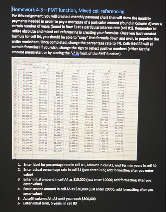
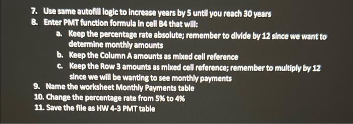
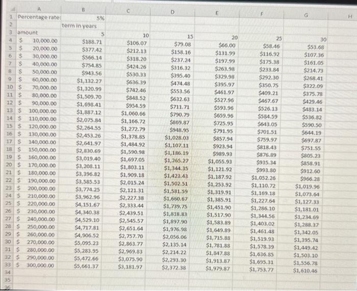
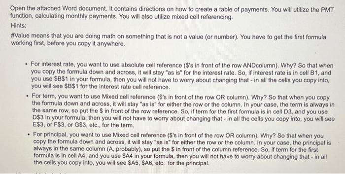
Homework 4-3 - PMT function, Mixed cell referencing For this assignment, you will create a monthly payment chart that will show the monthly payments needed in order to pay a mortgage of a particular amount (found in Column A) over a certain number of years (found in Row 3) at a particular interest rate (cell B1). Remember to utilize absolute and mixed cell referencing in creating your formulas, Once you have created formula for cell B4, you should be able to "copy" that formula down and over, to populate the entire worksheet. Once completed, change the percentage rate to 4%. Cells B4:G33 will all contain formulasi If you wish, change the sign to reflect positive numbers (elther for the amount parameter, or by placing the "." in front of the PMT function). 1. Enter label for percentage rate in cell A1, Amount in cell A3, and Term in years in cell B2 2. Enter actual percentage rate in call B1 (Just enter 0.05; add formatting after you enter value) 3. Enter initial amount in cell A4 as $10,000 (just enter 10000 ; add formatting after you enter value) 4. Enter second amount in cell A5 as $20,000 fust enter 20000 ; add formatting after you enter value) 5. Autofill column A4:A5 until you reach $300,000 6. Enter initial term, 5 years, in cell 83 7. Use same autofill logic to increase years by 5 until you reach 30 years 8. Enter PMT function formula in cell 84 that will: a. Keep the percentage rate absolute; remember to divide by 12 since we want to determine monthly amounts b. Keep the Column A amounts as mixed cell reference c. Keep the Row 3 amounts as mixed cell reference; remember to multiply by 12 since we will be wanting to see monthly payments 9. Name the worksheet Monthly Payments table 10. Change the percentage rate from 5% to 4% 11. Save the file as HW 4-3 PMT table Open the attached Word document. It contains directions on how to create a table of payments. You will utilize the PMT function, calculating monthly payments. You will also utilize mixed cell referencing. Hints: \#Value means that you are doing math on something that is not a value (or number). You have to get the first formula working first, before you copy it anywhere. - For interest rate, you want to use absolute cell reference (\$'s in front of the row ANDcolumn). Why? So that when you copy the formula down and across, it will stay "as is" for the interest rate. So, if interest rate is in cell B1, and you use $B$1 in your formula, then you will not have to worry about changing that - in all the cells you copy into, you will see $B$1 for the interest rate cell reference. - For term, you want to use Mixed cell reference (\$'s in front of the row OR column). Why? So that when you copy the formula down and across, it will stay "as is" for either the row or the column. In your case, the term is always in the same row, so put the $ in front of the row reference. So, if term for the first formula is in cell D3, and you use D $3 in your formula, then you will not have to worry about changing that - in all the cells you copy into, you will see E$3, or F$3, or G$3, etc., for the term. - For principal, you want to use Mixed cell reference ( $ 's in front of the row OR column). Why? So that when you copy the formula down and across, it will stay "as is" for either the row or the column. In your case, the principal is always in the same column ( A, probably), so put the $ in front of the column reference. So, if term for the first formula is in cell A4, and you use \$A4 in your formula, then you will not have to worry about changing that - in all the cells you copy into, you will see $A5,$A6, etc. for the principal. Homework 4-3 - PMT function, Mixed cell referencing For this assignment, you will create a monthly payment chart that will show the monthly payments needed in order to pay a mortgage of a particular amount (found in Column A) over a certain number of years (found in Row 3) at a particular interest rate (cell B1). Remember to utilize absolute and mixed cell referencing in creating your formulas, Once you have created formula for cell B4, you should be able to "copy" that formula down and over, to populate the entire worksheet. Once completed, change the percentage rate to 4%. Cells B4:G33 will all contain formulasi If you wish, change the sign to reflect positive numbers (elther for the amount parameter, or by placing the "." in front of the PMT function). 1. Enter label for percentage rate in cell A1, Amount in cell A3, and Term in years in cell B2 2. Enter actual percentage rate in call B1 (Just enter 0.05; add formatting after you enter value) 3. Enter initial amount in cell A4 as $10,000 (just enter 10000 ; add formatting after you enter value) 4. Enter second amount in cell A5 as $20,000 fust enter 20000 ; add formatting after you enter value) 5. Autofill column A4:A5 until you reach $300,000 6. Enter initial term, 5 years, in cell 83 7. Use same autofill logic to increase years by 5 until you reach 30 years 8. Enter PMT function formula in cell 84 that will: a. Keep the percentage rate absolute; remember to divide by 12 since we want to determine monthly amounts b. Keep the Column A amounts as mixed cell reference c. Keep the Row 3 amounts as mixed cell reference; remember to multiply by 12 since we will be wanting to see monthly payments 9. Name the worksheet Monthly Payments table 10. Change the percentage rate from 5% to 4% 11. Save the file as HW 4-3 PMT table Open the attached Word document. It contains directions on how to create a table of payments. You will utilize the PMT function, calculating monthly payments. You will also utilize mixed cell referencing. Hints: \#Value means that you are doing math on something that is not a value (or number). You have to get the first formula working first, before you copy it anywhere. - For interest rate, you want to use absolute cell reference (\$'s in front of the row ANDcolumn). Why? So that when you copy the formula down and across, it will stay "as is" for the interest rate. So, if interest rate is in cell B1, and you use $B$1 in your formula, then you will not have to worry about changing that - in all the cells you copy into, you will see $B$1 for the interest rate cell reference. - For term, you want to use Mixed cell reference (\$'s in front of the row OR column). Why? So that when you copy the formula down and across, it will stay "as is" for either the row or the column. In your case, the term is always in the same row, so put the $ in front of the row reference. So, if term for the first formula is in cell D3, and you use D $3 in your formula, then you will not have to worry about changing that - in all the cells you copy into, you will see E$3, or F$3, or G$3, etc., for the term. - For principal, you want to use Mixed cell reference ( $ 's in front of the row OR column). Why? So that when you copy the formula down and across, it will stay "as is" for either the row or the column. In your case, the principal is always in the same column ( A, probably), so put the $ in front of the column reference. So, if term for the first formula is in cell A4, and you use \$A4 in your formula, then you will not have to worry about changing that - in all the cells you copy into, you will see $A5,$A6, etc. for the principal