Hey please I just need you to show steps like how to do them because I dont know how to do it. PLEASE EXPLAIN LIKE YOURE EXPLAINING TO SOMEONE WHO NEVER USED EXCEL THANKS. STEPS 2-31.

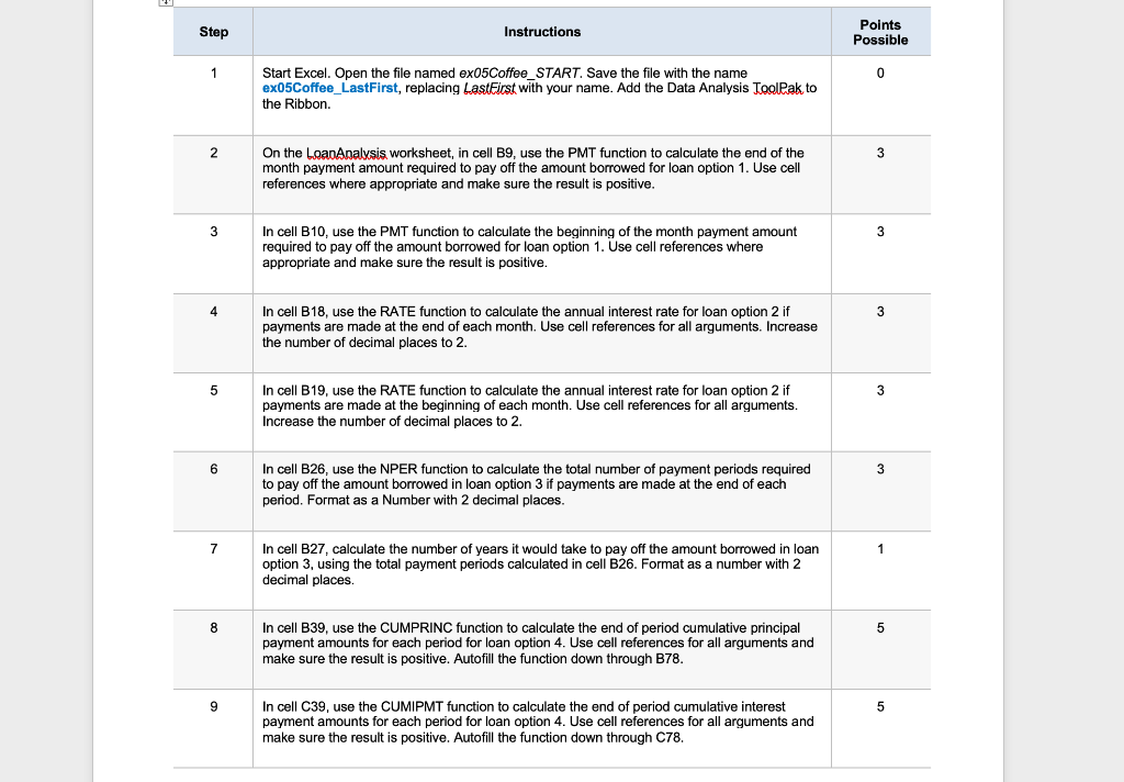
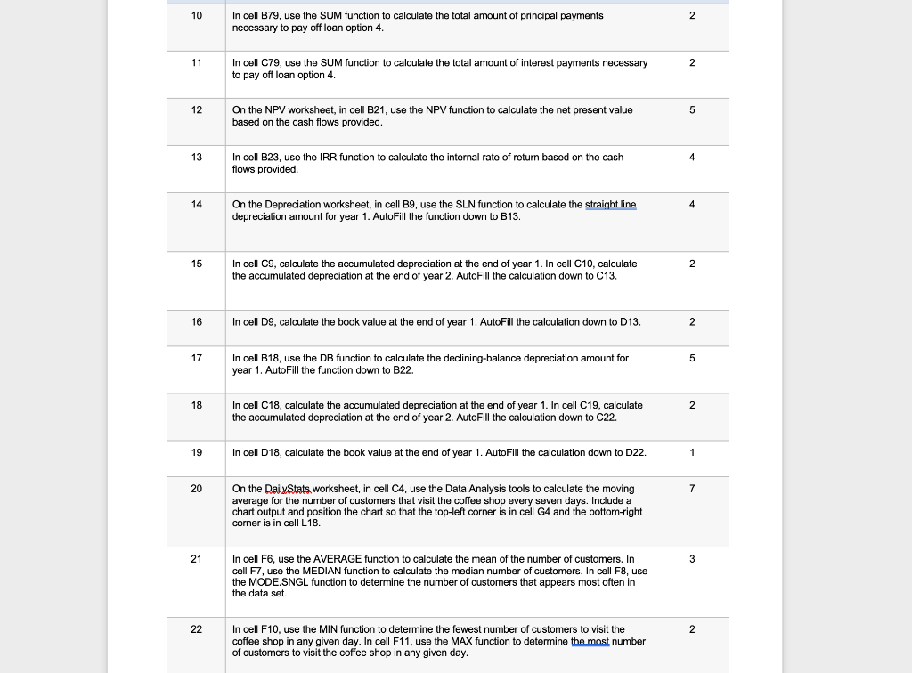
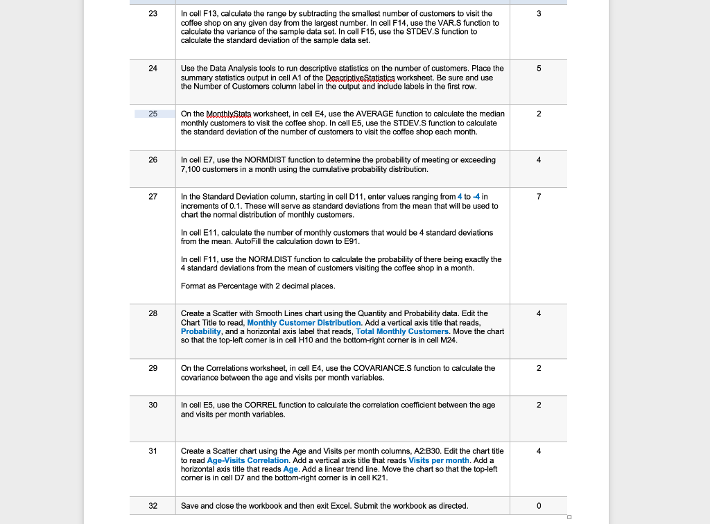
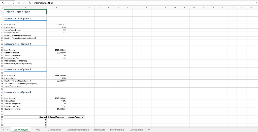
Step Instructions Points Possible 1 0 Start Excel. Open the file named ex05Coffee_START. Save the file with the name ex05Coffee_LastFirst, replacing LastFirst with your name. Add the Data Analysis ToolPak to the Ribbon. 2 3 On the Loan Analysis, worksheet, in cell B9, use the PMT function to calculate the end of the month payment amount required to pay off the amount borrowed for loan option 1. Use cell references where appropriate and make sure the result is positive. 3 3 In cell B10, use the PMT function to calculate the beginning of the month payment amount required to pay off the amount borrowed for loan option 1. Use cell references where appropriate and make sure the result is positive. 4 3 In cell B18, use the RATE function to calculate the annual interest rate for loan option 2 if payments are made at the end of each month. Use cell references for all arguments. Increase the number of decimal places to 2. 5 3 In cell B19, use the RATE function to calculate the annual interest rate for loan option 2 if payments are made at the beginning of each month. Use cell references for all arguments. Increase the number of decimal places to 2. 6 3 In cell B26, use the NPER function to calculate the total number of payment periods required to pay off the amount borrowed in loan option 3 if payments are made at the end of each period. Format as a Number with 2 decimal places. 7 1 In cell B27, calculate the number of years it would take to pay off the amount borrowed in loan option 3, using the total payment periods calculated in cell B26. Format as a number with 2 decimal places. 8 5 In cell B39, use the CUMPRINC function to calculate the end of period cumulative principal payment amounts for each period for loan option 4. Use cell references for all arguments and make sure the result is positive. Autofill function down through B78. 9 5 In cell C39, use the CUMIPMT function to calculate the end of period cumulative interest payment amounts for each period for loan option 4. Use cell references for all arguments and make sure the result is positive. Autofill the function down through C78. 10 2 2 In cell B79, use the SUM function to calculate the total amount of principal payments necessary to pay off loan option 4. 11 2 In cell C79, use the SUM function to calculate the total amount of interest payments necessary to pay off loan option 4. 12 5 On the NPV worksheet, in cell B21, use the NPV function to calculate the net present value based on the cash flows provided. 13 In cell B23, use the IRR function to calculate the internal rate of return based on the cash flows provided. 4 14 4 4 On the Depreciation worksheet, in cell B9, use the SLN function to calculate the straight line depreciation amount for year 1. AutoFill the function down to B13. 15 2 In cell C9, calculate the accumulated depreciation at the end of year 1. In cell C10, calculate the accumulated depreciation at the end of year 2. AutoFill the calculation down to C13. 16 In cell D9, calculate the book value at the end of year 1. AutoFill the calculation down to D13. 2 17 5 In cell B18, use the DB function to calculate the declining-balance depreciation amount for year 1. AutoFill the function down to B22. 18 2 In cell C18, calculate the accumulated depreciation at the end of year 1. In cell C19, calculate the accumulated depreciation at the end of year 2. AutoFill the calculation down to C22. 19 In cell D18, calculate the book value at the end of year 1. AutoFill the calculation down to D22. 1 20 7 On the Daily Stats, worksheet, in cell C4, use the Data Analysis tools to calculate the moving average for the number of customers that visit the coffee shop every seven days. Include a chart output and position the chart so that the top-left corner is in cell G4 and the bottom-right corner is in cell L18. 21 3 In cell F6, use the AVERAGE function to calculate the mean of the number of customers. In cell F7, use the MEDIAN function to calculate the median number of customers. In cell F8, use the MODE.SNGL function to determine the number of customers that appears most often in the data set. 22 2 In cell F10, use the MIN function to determine the fewest number of customers to visit the coffee shop in any given day. In cell F11, use the MAX function to determine the most number of customers to visit the coffee shop in any given day. 23 3 In cell F13, calculate the range by subtracting the smallest number of customers to visit the coffee shop on any given day from the largest number. In cell F14, use the VAR.S function to calculate the variance of the sample data set. In cell F15, use the STDEV.S function to calculate the standard deviation of the sample data set. 24 5 Use the Data Analysis tools to run descriptive statistics on the number of customers. Place the summary statistics output in cell A1 of the DescriptiveStatistics worksheet. Be sure and use the Number of Customers column label in the output and include labels in the first row. 25 2 On the MonthlyStats worksheet, in cell E4, use the AVERAGE function to calculate the median monthly customers to visit the coffee shop. In cell E5, use the STDEV.S function to calculate the standard deviation of the number of customers to visit the coffee shop each month. 26 4 In cell E7, use the NORMDIST function to determine the probability of meeting or exceeding 7,100 customers in a month using the cumulative probability distribution. 27 7 In the Standard Deviation column, starting in cell D11, enter values ranging from 4 to 4 in increments of 0.1. These will serve as standard deviations from the mean that will be used to chart the normal distribution of monthly customers. In cell E11, calculate the number of monthly customers that would be 4 standard deviations from the mean. AutoFill the calculation down to E91. In cell F11, use the NORM.DIST function to calculate the probability of there being exactly the 4 standard deviations from the mean of customers visiting the coffee shop in a month. Format as Percentage with 2 decimal places. 28 4 Create a Scatter with Smooth Lines chart using the Quantity and Probability data. Edit the Chart Title to read, Monthly Customer Distribution. Add a vertical axis title that reads, Probability, and a horizontal axis label that reads, Total Monthly Customers. Move the chart so that the top-left corner is in cell H10 and the bottom-right corner is in cell M24. 29 2 On the Correlations worksheet, in cell E4, use the COVARIANCE.S function to calculate the covariance between the age and visits per month variables. 30 2 In cell E5, use the CORREL function to calculate the correlation coefficient between the age and visits per month variables. 31 4 Create a Scatter chart using the Age and Visits per month columns, A2:B30. Edit the chart title to read Age-Visits Correlation. Add a vertical axis title that reads Visits per month. Add a horizontal axis title that reads Age. Add a linear trend line. Move the chart so that the top-left corner is in cell D7 and the bottom-right corner is in cell K21. 32 Save and close the workbook and then exit Excel. Submit the workbook as directed. 0 A1 1 x fx Chloe's Coffee Shop A C C D E F G H H 1 L L M N P u B S T U $ 210,000.00 7.20% 10 12 $210,000.00 $2,200.00 10 12 Chloe's Coffee Shop 2 Loan Analysis - Option 1 4 5 Laan Amount 5 6 Interest Rate 7 Term of Lour years) 8 Payments per Year 9 Monthly Payment (end of period 10 Monthly Payment beginning of period 11 12 Loan Analysis - Option 2 13 14 Laan Amount 15 Monthly Payment 16 Term of Loer veurs) 17 Payments per Year 18 Interest Rate (end of period 19 Interest Rate beginning of period 20 2. Loan Analysis - Option 3 22 23 Loan Amount 24 Interest Race 25 Monthly Payment (end of period 26 Tatal Number of Payments (end of period) 27 Term of loan in years 28 2s Loan Analysis - Option 4 30 31 Loan Amount 32 Interest Rate 33 term of Lour years) 34 Payments per les 35 Quarterly Payments 36 37 38 39 $210,000.00 7.20% $ $2,200.00 $218,000.00 7.2% 10 $7,692.29 Interest Payments Quarter Principal Payments 1 2 3 3 10 LoanAnalysis NPV Depreciation DescriptiveStatistics Daily Stats Monthly Stats Correlations + Al x fx Chloe's Coffee Shop D E F G E H K L M N N 0 P B S T U 37 39 40 42 42 43 44 45 46 97 48 49 50 51 52 53 54 SS 56 57 58 59 60 Quarter Principal Payments Interest Payments 1 2 3 4 5 6 7 8 9 in 11 ** 12 13 14 15 16 17 . 10 19 20 21 22 23 29 62 63 G4 65 25 2G 27 28 G7 68 69 29 30 31 70 32 33 34 35 36 37 72 73 74 75 76 77 78 79 80 39 39 40 Totals LoanAnalysis NPV Depreciation DescriptiveStatistics Daily Stats Monthly Stats Correlations + A1 2 x fc fx Chloe's Coffee Shop A C D E F H 1 x L M N P S s T v w Chloe's Coffee Shop 2 3 4 Discount Hate 3.50% 5 Total Initial Investment -$210,000.00 G 7 8 Cash Rows 9 Year0 $218,000.00 10 Year 1 $10,000.00 Year 2 $ 12,300.00 12 Year $15,100.00 13 Year 4 $15,600.00 14 Yaar E $22,800.00 15 Year G $ $25,100.00 16 Year $34,600.00 17 Year B $42,500.00 18 Year 9 $52,400.00 19 Year 10 $64,400.00 20 2: Net Present Value 22 23 Internal Rate of Return 24 25 26 27 28 20 30 31 32 33 34 35 32 38 39 40 42 43 LoanAnalysis NPV Depreciation DescriptiveStatistics Daily Stats Monthly Stats Correlations + A1 fx Chloe's Coffee Shop A C D F H 1 K L L M N N P S 1 U 1 Chloe's Coffee Shop 2 3 Cost of Asset 4 Salvage Value 5 Useful Life G 7 $24,000.00 $9,000.00 Straight Line Depreciation Depreciation Accumulated expense for depreciation a end of year 1 2 Book value at end of a End of Year year 3 9 10 10 12 13 14 15 16 Dedining-Balance Depredation Depreciation Accumulated expense for depreciation at End of Year ar end of year 1 2 Book value end of year 4 17 18 19 20 21 22 23 24 25 26 27 28 29 30 32 32 33 34 35 36 37 38 Loan Analysis NPV Depreciation DescriptiveStatistics Dailystals Monthly Stats Correlations + A1 A E E F G H 1 - N U R R S s 1 U V W X Y 2 1 2 3 4 5 6 7 9 10 11 12 13 14 15 16 17 18 20 21 22 23 24 26 27 28 25 30 31 32 33 34 35 36 37 38 39 40 42 43 44 LoanAnalysis NPV Depreciation Descriptive Statistics Daily Stats Monthly Stats Correlations + A1 x fx Chloe's Coffee Shop B E G H 1 1 K L M N P S T V w 1 Chloe's Coffee Shop Mean Median Mode Min Max Range Variance Standard Deviation 2 Day of the Number of Moving 3 3 Month Customen Average 4 1 143 2 153 6 3 43 6 3 132 7 178 5 166 3 c 9 6 154 10 7 123 1. 9 197 12 9 156 13 10 153 14 11 153 15 12 12 156 16 13 152 17 14 152 18 15 15 178 16 128 20 17 146 2 18 173 22 19 125 23 20 173 24 21 165 25 22 128 26 23 192 27 24 24 163 28 25 176 29 26 197 30 27 167 3: 28 188 32 29 165 33 30 182 34 31 122 36 37 38 39 40 41 41 LoanAnalysis NPV Depreciation DescriptiveStatistics Daily Stats Monthly Stats Correlations + A1 x fx Chloe's Coffee Shop A L H 1 j L M N P a R S T U 1 Chloe's Coffee Shop 2 Average Standard Deviation Desired Minimum Quantity Probability 7,100 Standard Deviation Quantity Probability 3 Month Total Customers 4 January 7,689 5 February 7,572 6 6 March 6,5R9 7 April 5,672 4,899 9 lure 4,374 10 July 5,638 11 August 6,583 12 September 7,203 13 October 7,753 14 November 2,878 15 December 8,112 16 17 18 19 20 20 22 23 24 25 26 27 28 29 30 3: 32 33 34 35 36 37 38 39 40 91 42 32 LoanAnalysis NPV Depreciation DescriptiveStatistics Daily Stats MonthlyStats Correlations + A1 . xfx Chloe's Coffee Shop B C E F G H 1 K L M N N 0 P R S T U V w Z 1 Coffee Shop Covariance Correlation 3 Visits per month 4 29 5 3 G 29 7 7 a 9 22 10 25 11 31 12 27 13 15 14 19 15 23 16 2 17 13 18 S 19 20 24 2 16 22 28 23 5 24 30 25 22 26 7 27 18 28 14 29 11 30 3 3 32 33 34 35 37 38 39 90 42 43 LoanAnalysis NPV Depreciation DescriptiveStatistics Daily Stats Monthly Stats Correlations + Step Instructions Points Possible 1 0 Start Excel. Open the file named ex05Coffee_START. Save the file with the name ex05Coffee_LastFirst, replacing LastFirst with your name. Add the Data Analysis ToolPak to the Ribbon. 2 3 On the Loan Analysis, worksheet, in cell B9, use the PMT function to calculate the end of the month payment amount required to pay off the amount borrowed for loan option 1. Use cell references where appropriate and make sure the result is positive. 3 3 In cell B10, use the PMT function to calculate the beginning of the month payment amount required to pay off the amount borrowed for loan option 1. Use cell references where appropriate and make sure the result is positive. 4 3 In cell B18, use the RATE function to calculate the annual interest rate for loan option 2 if payments are made at the end of each month. Use cell references for all arguments. Increase the number of decimal places to 2. 5 3 In cell B19, use the RATE function to calculate the annual interest rate for loan option 2 if payments are made at the beginning of each month. Use cell references for all arguments. Increase the number of decimal places to 2. 6 3 In cell B26, use the NPER function to calculate the total number of payment periods required to pay off the amount borrowed in loan option 3 if payments are made at the end of each period. Format as a Number with 2 decimal places. 7 1 In cell B27, calculate the number of years it would take to pay off the amount borrowed in loan option 3, using the total payment periods calculated in cell B26. Format as a number with 2 decimal places. 8 5 In cell B39, use the CUMPRINC function to calculate the end of period cumulative principal payment amounts for each period for loan option 4. Use cell references for all arguments and make sure the result is positive. Autofill function down through B78. 9 5 In cell C39, use the CUMIPMT function to calculate the end of period cumulative interest payment amounts for each period for loan option 4. Use cell references for all arguments and make sure the result is positive. Autofill the function down through C78. 10 2 2 In cell B79, use the SUM function to calculate the total amount of principal payments necessary to pay off loan option 4. 11 2 In cell C79, use the SUM function to calculate the total amount of interest payments necessary to pay off loan option 4. 12 5 On the NPV worksheet, in cell B21, use the NPV function to calculate the net present value based on the cash flows provided. 13 In cell B23, use the IRR function to calculate the internal rate of return based on the cash flows provided. 4 14 4 4 On the Depreciation worksheet, in cell B9, use the SLN function to calculate the straight line depreciation amount for year 1. AutoFill the function down to B13. 15 2 In cell C9, calculate the accumulated depreciation at the end of year 1. In cell C10, calculate the accumulated depreciation at the end of year 2. AutoFill the calculation down to C13. 16 In cell D9, calculate the book value at the end of year 1. AutoFill the calculation down to D13. 2 17 5 In cell B18, use the DB function to calculate the declining-balance depreciation amount for year 1. AutoFill the function down to B22. 18 2 In cell C18, calculate the accumulated depreciation at the end of year 1. In cell C19, calculate the accumulated depreciation at the end of year 2. AutoFill the calculation down to C22. 19 In cell D18, calculate the book value at the end of year 1. AutoFill the calculation down to D22. 1 20 7 On the Daily Stats, worksheet, in cell C4, use the Data Analysis tools to calculate the moving average for the number of customers that visit the coffee shop every seven days. Include a chart output and position the chart so that the top-left corner is in cell G4 and the bottom-right corner is in cell L18. 21 3 In cell F6, use the AVERAGE function to calculate the mean of the number of customers. In cell F7, use the MEDIAN function to calculate the median number of customers. In cell F8, use the MODE.SNGL function to determine the number of customers that appears most often in the data set. 22 2 In cell F10, use the MIN function to determine the fewest number of customers to visit the coffee shop in any given day. In cell F11, use the MAX function to determine the most number of customers to visit the coffee shop in any given day. 23 3 In cell F13, calculate the range by subtracting the smallest number of customers to visit the coffee shop on any given day from the largest number. In cell F14, use the VAR.S function to calculate the variance of the sample data set. In cell F15, use the STDEV.S function to calculate the standard deviation of the sample data set. 24 5 Use the Data Analysis tools to run descriptive statistics on the number of customers. Place the summary statistics output in cell A1 of the DescriptiveStatistics worksheet. Be sure and use the Number of Customers column label in the output and include labels in the first row. 25 2 On the MonthlyStats worksheet, in cell E4, use the AVERAGE function to calculate the median monthly customers to visit the coffee shop. In cell E5, use the STDEV.S function to calculate the standard deviation of the number of customers to visit the coffee shop each month. 26 4 In cell E7, use the NORMDIST function to determine the probability of meeting or exceeding 7,100 customers in a month using the cumulative probability distribution. 27 7 In the Standard Deviation column, starting in cell D11, enter values ranging from 4 to 4 in increments of 0.1. These will serve as standard deviations from the mean that will be used to chart the normal distribution of monthly customers. In cell E11, calculate the number of monthly customers that would be 4 standard deviations from the mean. AutoFill the calculation down to E91. In cell F11, use the NORM.DIST function to calculate the probability of there being exactly the 4 standard deviations from the mean of customers visiting the coffee shop in a month. Format as Percentage with 2 decimal places. 28 4 Create a Scatter with Smooth Lines chart using the Quantity and Probability data. Edit the Chart Title to read, Monthly Customer Distribution. Add a vertical axis title that reads, Probability, and a horizontal axis label that reads, Total Monthly Customers. Move the chart so that the top-left corner is in cell H10 and the bottom-right corner is in cell M24. 29 2 On the Correlations worksheet, in cell E4, use the COVARIANCE.S function to calculate the covariance between the age and visits per month variables. 30 2 In cell E5, use the CORREL function to calculate the correlation coefficient between the age and visits per month variables. 31 4 Create a Scatter chart using the Age and Visits per month columns, A2:B30. Edit the chart title to read Age-Visits Correlation. Add a vertical axis title that reads Visits per month. Add a horizontal axis title that reads Age. Add a linear trend line. Move the chart so that the top-left corner is in cell D7 and the bottom-right corner is in cell K21. 32 Save and close the workbook and then exit Excel. Submit the workbook as directed. 0 A1 1 x fx Chloe's Coffee Shop A C C D E F G H H 1 L L M N P u B S T U $ 210,000.00 7.20% 10 12 $210,000.00 $2,200.00 10 12 Chloe's Coffee Shop 2 Loan Analysis - Option 1 4 5 Laan Amount 5 6 Interest Rate 7 Term of Lour years) 8 Payments per Year 9 Monthly Payment (end of period 10 Monthly Payment beginning of period 11 12 Loan Analysis - Option 2 13 14 Laan Amount 15 Monthly Payment 16 Term of Loer veurs) 17 Payments per Year 18 Interest Rate (end of period 19 Interest Rate beginning of period 20 2. Loan Analysis - Option 3 22 23 Loan Amount 24 Interest Race 25 Monthly Payment (end of period 26 Tatal Number of Payments (end of period) 27 Term of loan in years 28 2s Loan Analysis - Option 4 30 31 Loan Amount 32 Interest Rate 33 term of Lour years) 34 Payments per les 35 Quarterly Payments 36 37 38 39 $210,000.00 7.20% $ $2,200.00 $218,000.00 7.2% 10 $7,692.29 Interest Payments Quarter Principal Payments 1 2 3 3 10 LoanAnalysis NPV Depreciation DescriptiveStatistics Daily Stats Monthly Stats Correlations + Al x fx Chloe's Coffee Shop D E F G E H K L M N N 0 P B S T U 37 39 40 42 42 43 44 45 46 97 48 49 50 51 52 53 54 SS 56 57 58 59 60 Quarter Principal Payments Interest Payments 1 2 3 4 5 6 7 8 9 in 11 ** 12 13 14 15 16 17 . 10 19 20 21 22 23 29 62 63 G4 65 25 2G 27 28 G7 68 69 29 30 31 70 32 33 34 35 36 37 72 73 74 75 76 77 78 79 80 39 39 40 Totals LoanAnalysis NPV Depreciation DescriptiveStatistics Daily Stats Monthly Stats Correlations + A1 2 x fc fx Chloe's Coffee Shop A C D E F H 1 x L M N P S s T v w Chloe's Coffee Shop 2 3 4 Discount Hate 3.50% 5 Total Initial Investment -$210,000.00 G 7 8 Cash Rows 9 Year0 $218,000.00 10 Year 1 $10,000.00 Year 2 $ 12,300.00 12 Year $15,100.00 13 Year 4 $15,600.00 14 Yaar E $22,800.00 15 Year G $ $25,100.00 16 Year $34,600.00 17 Year B $42,500.00 18 Year 9 $52,400.00 19 Year 10 $64,400.00 20 2: Net Present Value 22 23 Internal Rate of Return 24 25 26 27 28 20 30 31 32 33 34 35 32 38 39 40 42 43 LoanAnalysis NPV Depreciation DescriptiveStatistics Daily Stats Monthly Stats Correlations + A1 fx Chloe's Coffee Shop A C D F H 1 K L L M N N P S 1 U 1 Chloe's Coffee Shop 2 3 Cost of Asset 4 Salvage Value 5 Useful Life G 7 $24,000.00 $9,000.00 Straight Line Depreciation Depreciation Accumulated expense for depreciation a end of year 1 2 Book value at end of a End of Year year 3 9 10 10 12 13 14 15 16 Dedining-Balance Depredation Depreciation Accumulated expense for depreciation at End of Year ar end of year 1 2 Book value end of year 4 17 18 19 20 21 22 23 24 25 26 27 28 29 30 32 32 33 34 35 36 37 38 Loan Analysis NPV Depreciation DescriptiveStatistics Dailystals Monthly Stats Correlations + A1 A E E F G H 1 - N U R R S s 1 U V W X Y 2 1 2 3 4 5 6 7 9 10 11 12 13 14 15 16 17 18 20 21 22 23 24 26 27 28 25 30 31 32 33 34 35 36 37 38 39 40 42 43 44 LoanAnalysis NPV Depreciation Descriptive Statistics Daily Stats Monthly Stats Correlations + A1 x fx Chloe's Coffee Shop B E G H 1 1 K L M N P S T V w 1 Chloe's Coffee Shop Mean Median Mode Min Max Range Variance Standard Deviation 2 Day of the Number of Moving 3 3 Month Customen Average 4 1 143 2 153 6 3 43 6 3 132 7 178 5 166 3 c 9 6 154 10 7 123 1. 9 197 12 9 156 13 10 153 14 11 153 15 12 12 156 16 13 152 17 14 152 18 15 15 178 16 128 20 17 146 2 18 173 22 19 125 23 20 173 24 21 165 25 22 128 26 23 192 27 24 24 163 28 25 176 29 26 197 30 27 167 3: 28 188 32 29 165 33 30 182 34 31 122 36 37 38 39 40 41 41 LoanAnalysis NPV Depreciation DescriptiveStatistics Daily Stats Monthly Stats Correlations + A1 x fx Chloe's Coffee Shop A L H 1 j L M N P a R S T U 1 Chloe's Coffee Shop 2 Average Standard Deviation Desired Minimum Quantity Probability 7,100 Standard Deviation Quantity Probability 3 Month Total Customers 4 January 7,689 5 February 7,572 6 6 March 6,5R9 7 April 5,672 4,899 9 lure 4,374 10 July 5,638 11 August 6,583 12 September 7,203 13 October 7,753 14 November 2,878 15 December 8,112 16 17 18 19 20 20 22 23 24 25 26 27 28 29 30 3: 32 33 34 35 36 37 38 39 40 91 42 32 LoanAnalysis NPV Depreciation DescriptiveStatistics Daily Stats MonthlyStats Correlations + A1 . xfx Chloe's Coffee Shop B C E F G H 1 K L M N N 0 P R S T U V w Z 1 Coffee Shop Covariance Correlation 3 Visits per month 4 29 5 3 G 29 7 7 a 9 22 10 25 11 31 12 27 13 15 14 19 15 23 16 2 17 13 18 S 19 20 24 2 16 22 28 23 5 24 30 25 22 26 7 27 18 28 14 29 11 30 3 3 32 33 34 35 37 38 39 90 42 43 LoanAnalysis NPV Depreciation DescriptiveStatistics Daily Stats Monthly Stats Correlations +