How do I make window sizes in matlab? And then how do I implement these functions into the code?

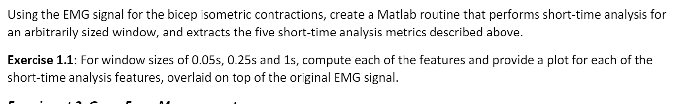
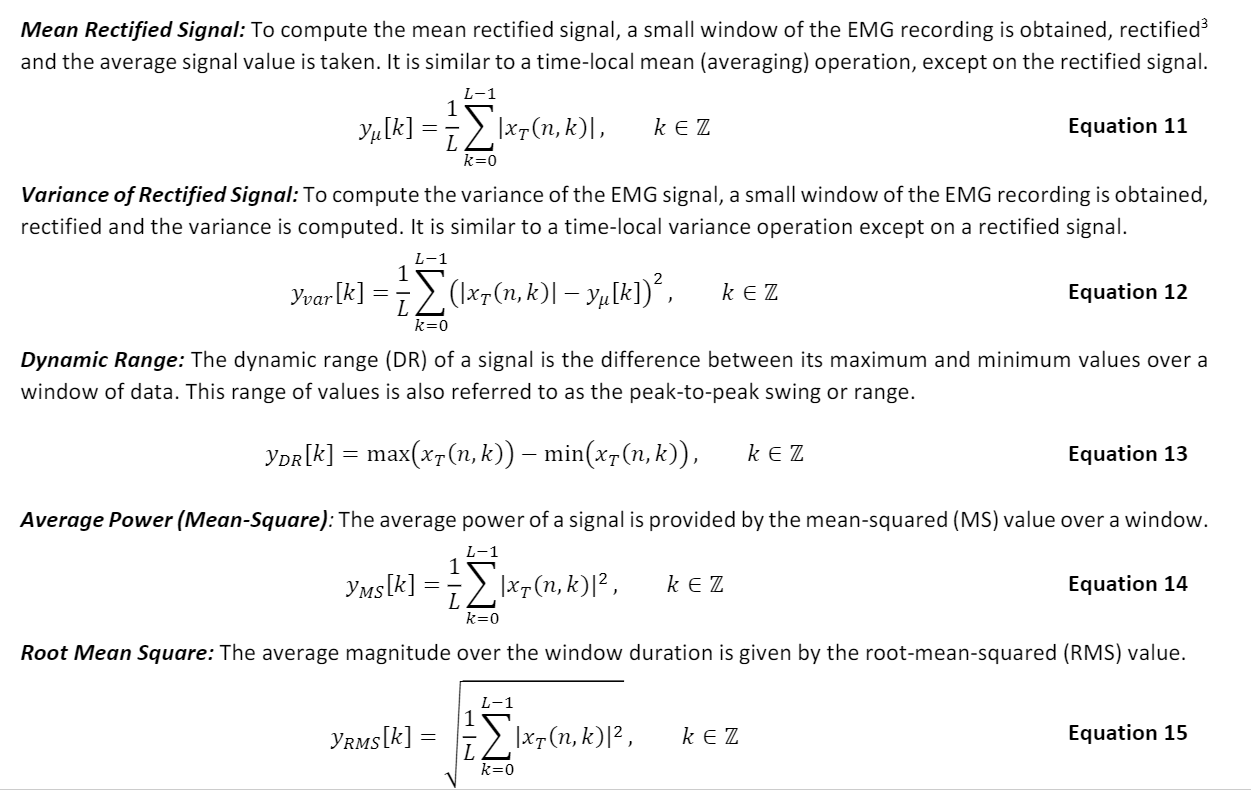
Using the EMG signal for the bicep isometric contractions, create a Matlab routine that performs short-time analysis for an arbitrarily sized window, and extracts the five short-time analysis metrics described above. Exercise 1.1: For window sizes of 0.05s, 0.25s and 1s, compute each of the features and provide a plot for each of the short-time analysis features, overlaid on top of the original EMG signal. Mean Rectified Signal: To compute the mean rectified signal, a small window of the EMG recording is obtained, rectified and the average signal value is taken. It is similar to a time-local mean (averaging) operation, except on the rectified signal. L-1 k EZ Equation 11 Yu [k] {ixo[n, k), k=0 Variance of Rectified Signal: To compute the variance of the EMG signal, a small window of the EMG recording is obtained, rectified and the variance is computed. It is similar to a time-local variance operation except on a rectified signal. L-1 Yvar[k] (1x7(n,k)] yp[k])?, k EZ Equation 12 k=0 Dynamic Range: The dynamic range (DR) of a signal is the difference between its maximum and minimum values over a window of data. This range of values is also referred to as the peak-to-peak swing or range. Ydr[k] = max(x7(n,k)) - min(x7(n,k)), k EZ Equation 13 Average Power (Mean-Square): The average power of a signal is provided by the mean-squared (MS) value over a window. L-1 1 Yms[k] *} \xy (,k)l2, k EZ Equation 14 L k=0 Root Mean Square: The average magnitude over the window duration is given by the root-mean-squared (RMS) value. L-1 Vras[k] = ixz (n, k)l2, k EZ Equation 15 k=0 Using the EMG signal for the bicep isometric contractions, create a Matlab routine that performs short-time analysis for an arbitrarily sized window, and extracts the five short-time analysis metrics described above. Exercise 1.1: For window sizes of 0.05s, 0.25s and 1s, compute each of the features and provide a plot for each of the short-time analysis features, overlaid on top of the original EMG signal. Mean Rectified Signal: To compute the mean rectified signal, a small window of the EMG recording is obtained, rectified and the average signal value is taken. It is similar to a time-local mean (averaging) operation, except on the rectified signal. L-1 k EZ Equation 11 Yu [k] {ixo[n, k), k=0 Variance of Rectified Signal: To compute the variance of the EMG signal, a small window of the EMG recording is obtained, rectified and the variance is computed. It is similar to a time-local variance operation except on a rectified signal. L-1 Yvar[k] (1x7(n,k)] yp[k])?, k EZ Equation 12 k=0 Dynamic Range: The dynamic range (DR) of a signal is the difference between its maximum and minimum values over a window of data. This range of values is also referred to as the peak-to-peak swing or range. Ydr[k] = max(x7(n,k)) - min(x7(n,k)), k EZ Equation 13 Average Power (Mean-Square): The average power of a signal is provided by the mean-squared (MS) value over a window. L-1 1 Yms[k] *} \xy (,k)l2, k EZ Equation 14 L k=0 Root Mean Square: The average magnitude over the window duration is given by the root-mean-squared (RMS) value. L-1 Vras[k] = ixz (n, k)l2, k EZ Equation 15 k=0