how do make the coulmn look like that ?

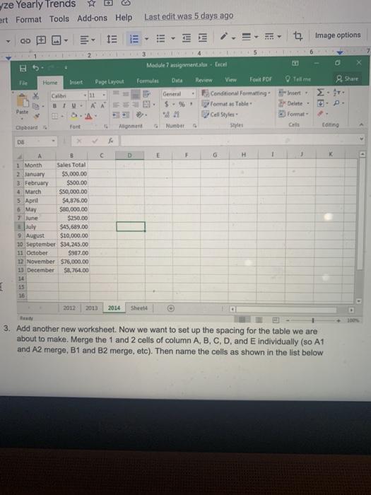
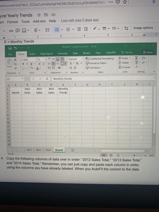
ze Yearly Trends ert Format Tools Add-ons Help Last edit was 5 days ago CD 15 E Image options 6 B Module 7 assignments Encel Home Pie Formula Page Layout Data Tell me 2. Share 2. Calin AAS General 5. 21 Number Review View Fond PDF Conditional Formatting Formats Table Cell Styles Styles Insert - Delete- E Format G Paste S.A. Clipboard font Am Editing DO 4 C. D E F G H 1 B 1 Month Sales Total 2 January $5,000.00 3. February $500.00 4 March $50,000.00 5 April $4,876.00 6. May $80,000.00 $250.00 July $45,689.00 9. August $10,000.00 10 September $34,245.00 11 October $987.00 12 November 576,000.00 December $8,764.00 14 7 June E 16 2012 2013 2014 Sheet 3. Add another new worksheet. Now we want to set up the spacing for the table we are about to make. Merge the 1 and 2 cells of column A, B, C, D, and individually (so A1 and A2 merge, B1 and B2 merge, etc). Then name the cells as shown in the list below o /document/d/1kb1_ZoZeZuXHbQ4qFNK38r2GdCUcLYFOHIWfETIYIW yze Yearly Trends #b ert Format Tools Add-ons Help Last edit was 5 days ago IEE image options 5 6 7 1 E = Monthly Trends Module 7 ansambel File Tell me Insert Formulas Home Data Shure Page Layout 11 AA Calibri 3 IV- 2. General $ - Review View Four PDF Po Conditional Formatting Format w Table Cell Styles Insert Delete- Format - SA De Font Alignment Number Editing El > Monthly Trends F G H 1 K 5 2012 Sales C 2013 Sales D 2014 Sales Monthly Trends Month 1 2 3 4 5 7 8 10 11 13 14 15 16 2013 2014 Shelt Sheet 100% 4. Copy the following columns of data over in order: "2012 Sales Total, 2013 Sales Total," and "2014 Sales Total. Remember, you can just copy and paste each column in order, using the columns you have already labeled. When you AutoFit the column to the data ze Yearly Trends ert Format Tools Add-ons Help Last edit was 5 days ago CD 15 E Image options 6 B Module 7 assignments Encel Home Pie Formula Page Layout Data Tell me 2. Share 2. Calin AAS General 5. 21 Number Review View Fond PDF Conditional Formatting Formats Table Cell Styles Styles Insert - Delete- E Format G Paste S.A. Clipboard font Am Editing DO 4 C. D E F G H 1 B 1 Month Sales Total 2 January $5,000.00 3. February $500.00 4 March $50,000.00 5 April $4,876.00 6. May $80,000.00 $250.00 July $45,689.00 9. August $10,000.00 10 September $34,245.00 11 October $987.00 12 November 576,000.00 December $8,764.00 14 7 June E 16 2012 2013 2014 Sheet 3. Add another new worksheet. Now we want to set up the spacing for the table we are about to make. Merge the 1 and 2 cells of column A, B, C, D, and individually (so A1 and A2 merge, B1 and B2 merge, etc). Then name the cells as shown in the list below o /document/d/1kb1_ZoZeZuXHbQ4qFNK38r2GdCUcLYFOHIWfETIYIW yze Yearly Trends #b ert Format Tools Add-ons Help Last edit was 5 days ago IEE image options 5 6 7 1 E = Monthly Trends Module 7 ansambel File Tell me Insert Formulas Home Data Shure Page Layout 11 AA Calibri 3 IV- 2. General $ - Review View Four PDF Po Conditional Formatting Format w Table Cell Styles Insert Delete- Format - SA De Font Alignment Number Editing El > Monthly Trends F G H 1 K 5 2012 Sales C 2013 Sales D 2014 Sales Monthly Trends Month 1 2 3 4 5 7 8 10 11 13 14 15 16 2013 2014 Shelt Sheet 100% 4. Copy the following columns of data over in order: "2012 Sales Total, 2013 Sales Total," and "2014 Sales Total. Remember, you can just copy and paste each column in order, using the columns you have already labeled. When you AutoFit the column to the data