HW02: PCM for Sound Processing

Start from file pcmencdec_hw2.m. Run the code step by step make sure you understand how it works and then

pcmencdec_hw2.m

% ============ % PCM ENCODING % ============ % from https://www.mathworks.com/matlabcentral/fileexchange/34610-pcm-matlab-code/content/Untitled.m % modified by JEC for CSE408 HW2

clc; clear all;

f = 3; % input frequency 3Hz

fs = 20; % sampling at 20Hz Ts = 1/fs; % sampling period = 1/fs

fss = 1.e4; % fine sampling for a pseudo-continuous time axis 10k sampls/sec Tss = 1/fss;

t = 0:Tss:2-Tss; % create a pseudo-continuous time axis, 2 seconds, 20k samples d = Ts/40:Ts:2+Ts/40; % discrete time axis: 41 samples starting at... % a very small value, 1/40 of the Sampling Period % rectangular pulses 1/Ts wide are 20 samples (1/fs*25)/(1/Tss)) wide in the t scale (which % is 10000Hz, while fs is 20Hz p = pulstran(t,d,'rectpuls',1/(fs*25));

% ================= % Analog MSG Signal % ================= % simple sinusoid at f (2fps) with a +shift of 1.1 to keep all values above % zero m = sin(2*pi*f*t)+1.1; % constant 1.1 is added so all values are positive % HW part 3 % comment the line above (and assign a new value to it) % add 1Hz 25% amplitude modulation to the input m, i.e. positive % amplitude variation between 0.75 and 1.25 % Hint: the modulating sin or cos amplitude is 0.25, so you need to add 1.0 % observe the reconstructed signal, why is it not correct? % what adjustment do you need to do to the signal so the dynamic range % remains as before? % insert your code here..

% ================= % Sampled signal % ================= ms = m.*p;

% ================= % Quantized Msg % ================= qm = quant(ms,2/16); em = 8*(qm);

% ================= % ENCODING MSG % =================

% get the sampled signal j = 1; for i=1:length(em) if (em(i)~=0 && em(i-1)==0) || ((i==1)&&(em(i)~=0)) x(j) = em(i)-1; j=j+1; end end

% convert to binary representation z = dec2bin(x,5); z = z'; z = z(:); z = str2num(z);

% z is the binary string sent through the channel, using 5-bit symbols

% ============= % PCM DE-CODING % ============= % the input is z % we know in advance that the stream is made of 5-bit symbols rb = z; l = length(rb);

for i = 1:l/5 q = rb((5*i)-4:5*i); q = num2str(q'); x1(i) = bin2dec(q); e(i) = x1(i)+1; end

dm = e/8; % decoded message signal

% Now recover the original signal by interpolating e using % fs*upSamplingFactor samples upSamplingFactor = 2;

rm = interpft(dm,fs*upSamplingFactor); % This is the received signal

% define discrete time axis for recovered signal Tsr = 2*Ts/upSamplingFactor; dr = 0:Tsr:2-Tsr;

% ================== % Plotting Signals % ==================

% uncomment to look at intermediate signals and for debugging figure(1); subplot(2,1,1) plot(t,m,'b',t,ms,'r'); legend('Analog Msg','Sampled Msg') grid; xlabel('t -->'); ylabel('Amplitude'); axis([0 2 0 2.25]);

subplot(2,1,2) plot(t,ms,'k',t,qm,'r'); legend('Sampled Msg','Quantized Msg') grid; xlabel('t -->'); ylabel('Amplitude'); axis([0 2 0 2.25]);

figure(2); %subplot(2,1,1) plot(t,em,'b') xlabel('t -->'); ylabel('Amplitude'); title('Encoded Msg sent'); grid; axis([0 2 -0.5 16.5]);

figure(3); stem(rm,'Marker','.'); title('Recovered Sampled Msg') grid; xlabel('t -->'); ylabel('Amplitude');

figure; plot(t,m,'b'); title('Original Signal') grid; xlabel('t -->'); ylabel('Amplitude'); axis([0 2 0 2.25]);

figure; plot(dr,rm,'b'); title('Recovered Analog Msg') grid; xlabel('t -->'); ylabel('Amplitude'); axis([0 2 0 2.25]);

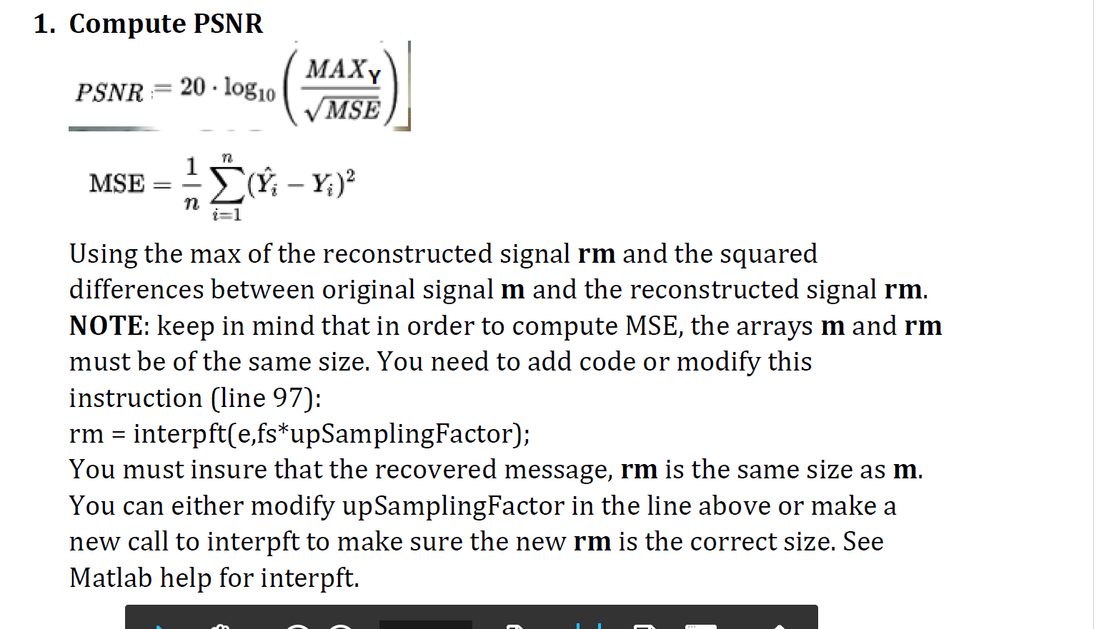
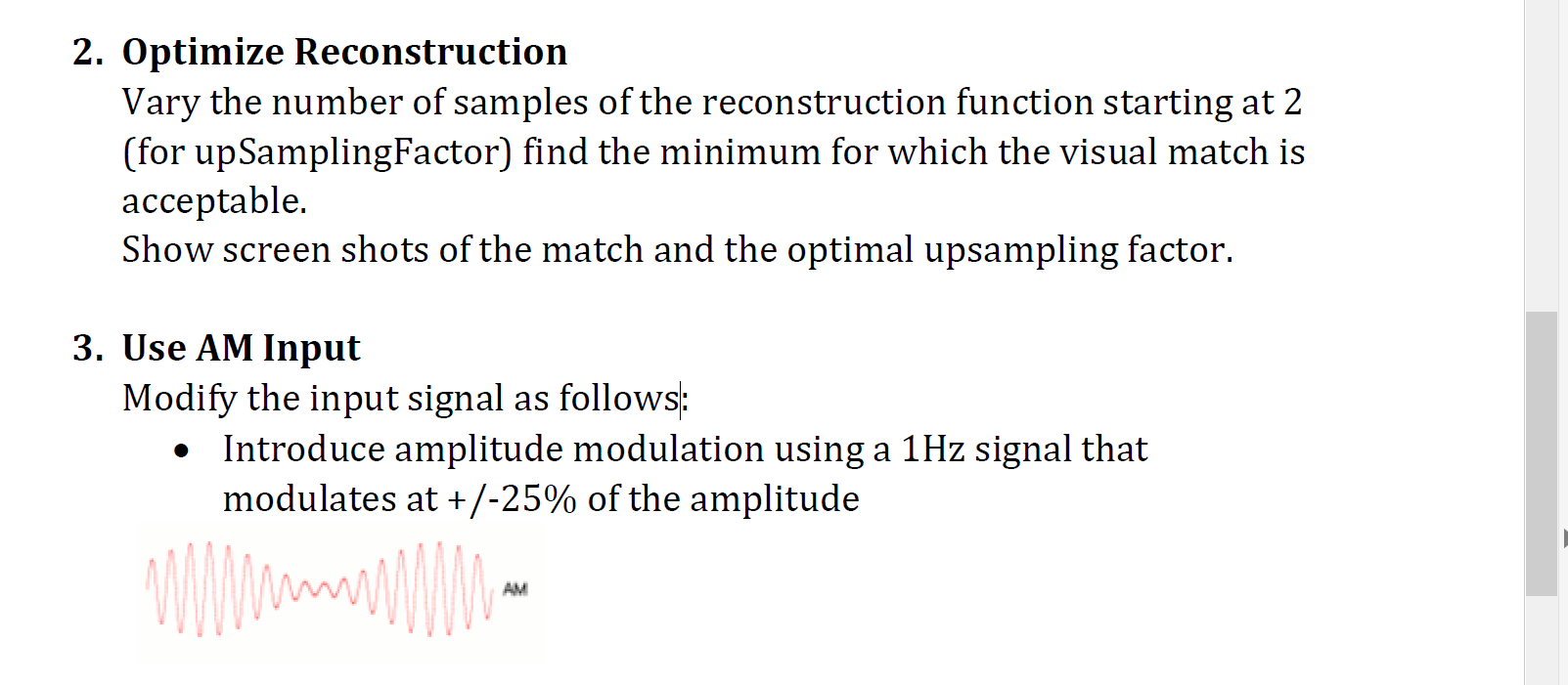
1. Compute PSNR PSNR = 20 log10 MAX , MSE ( l : Y;) n MSE n i=1 Using the max of the reconstructed signal rm and the squared differences between original signal m and the reconstructed signal rm. NOTE: keep in mind that in order to compute MSE, the arrays m and rm must be of the same size. You need to add code or modify this instruction (line 97): rm = interpft(e,fs*upSamplingFactor); You must insure that the recovered message, rm is the same size as m. You can either modify upSamplingFactor in the line above or make a new call to interpft to make sure the new rm is the correct size. See Matlab help for interpft. 2. Optimize Reconstruction Vary the number of samples of the reconstruction function starting at 2 (for upSamplingFactor) find the minimum for which the visual match is acceptable. Show screen shots of the match and the optimal upsampling factor. 3. Use AM Input Modify the input signal as follows: Introduce amplitude modulation using a 1Hz signal that modulates at +/-25% of the amplitude AM Compute the new PSNR. 4. Repeat step 2 for the AM Input Show screen shots of the match and the optimal upsampling factor. 1. Compute PSNR PSNR = 20 log10 MAX , MSE ( l : Y;) n MSE n i=1 Using the max of the reconstructed signal rm and the squared differences between original signal m and the reconstructed signal rm. NOTE: keep in mind that in order to compute MSE, the arrays m and rm must be of the same size. You need to add code or modify this instruction (line 97): rm = interpft(e,fs*upSamplingFactor); You must insure that the recovered message, rm is the same size as m. You can either modify upSamplingFactor in the line above or make a new call to interpft to make sure the new rm is the correct size. See Matlab help for interpft. 2. Optimize Reconstruction Vary the number of samples of the reconstruction function starting at 2 (for upSamplingFactor) find the minimum for which the visual match is acceptable. Show screen shots of the match and the optimal upsampling factor. 3. Use AM Input Modify the input signal as follows: Introduce amplitude modulation using a 1Hz signal that modulates at +/-25% of the amplitude AM Compute the new PSNR. 4. Repeat step 2 for the AM Input Show screen shots of the match and the optimal upsampling factor