I AM LOOKING FOR THE SOLUTIONS TO THESE PROBLEMS ON EXCEL. PLEASE GIVE DETAILED FORMULAS AND HOW TO SOLVE THE PROBLEMS. THANK YOU!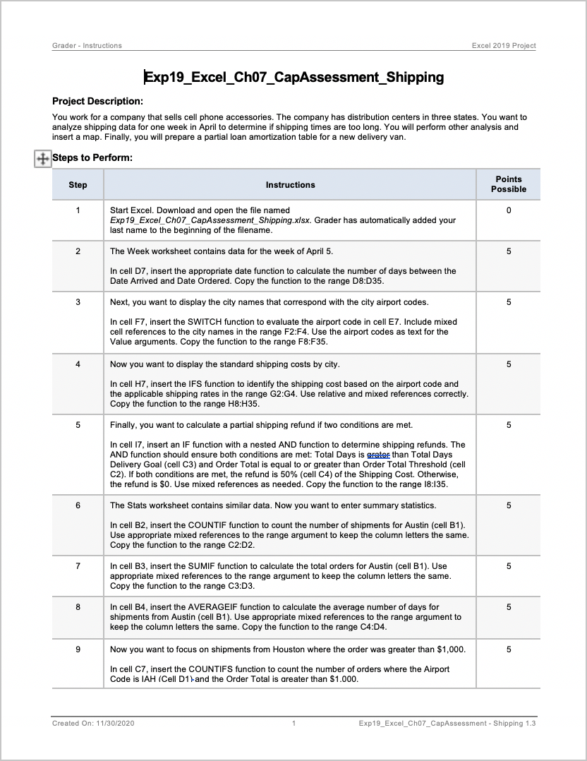

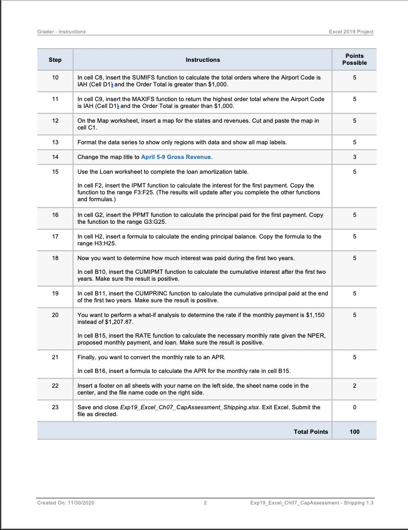
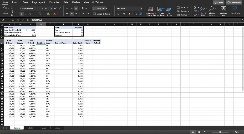
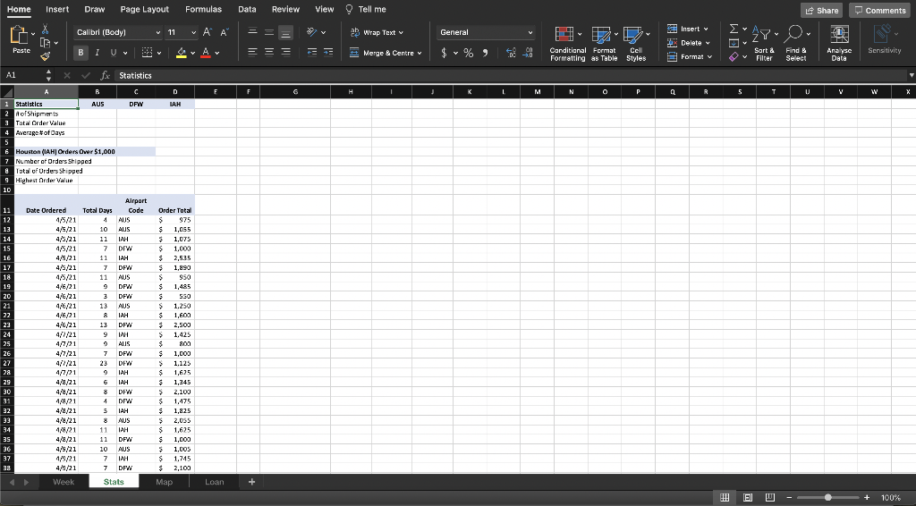
Grader - Instructions Excel 2019 Project Exp19_Excel_Ch07_CapAssessment_Shipping Project Description: You work for a company that sells cell phone accessories. The company has distribution centers in three states. You want to analyze shipping data for one week in April to determine if shipping times are too long. You will perform other analysis and insert a map. Finally, you will prepare a partial loan amortization table for a new delivery van. + Steps to Perform: Step Instructions Points Possible 1 0 Start Excel. Download and open the file named Exp19_Excel_Cho7_CapAssessment_Shipping.xlsx. Grader has automatically added your last name to the beginning of the filename. 2 The Week worksheet contains data for the week of April 5. 5 In cell D7, insert the appropriate date function to calculate the number of days between the Date Arrived and Date Ordered. Copy the function to the range 08:D35. 3 Next, you want to display the city names that correspond with the city airport codes. 5 In cell F7, insert the SWITCH function to evaluate the airport code in cell E7. Include mixed cell references to the city names in the range F2:F4. Use the airport codes as text for the Value arguments. Copy the function to the range F8:F35. 4 5 Now you want to display the standard shipping costs by city. In cell H7, insert the IFS function to identify the shipping cost based on the airport code and the applicable shipping rates in the range G2:44. Use relative and mixed references correctly. Copy the function to the range H8:H35. 5 Finally, you want to calculate a partial shipping refund if two conditions are met. 5 In cell 17, insert an IF function with a nested AND function to determine shipping refunds. The AND function should ensure both conditions are met: Total Days is skater than Total Days Delivery Goal (cell C3) and Order Total is equal to or greater than Order Total Threshold (cell C2). If both conditions are met, the refund is 50% (cell C4) of the Shipping Cost. Otherwise, the refund is $0. Use mixed references as needed. Copy the function to the range 18:135. 6 5 The Stats worksheet contains similar data. Now you want to enter summary statistics. In cell B2, insert the COUNTIF function to count the number of shipments for Austin (cell B1). Use appropriate mixed references to the range argument to keep the column letters the same. Copy the function to the range C2:D2. 7 5 In cell B3, insert the SUMIF function to calculate the total orders for Austin (cell B1). Use appropriate mixed references to the range argument to keep the column letters the same. Copy the function to the range C3:D3. 8 5 In cell B4, insert the AVERAGEIF function to calculate the average number of days for shipm rom Austin (cell B1). Use mixed references to the range argument to keep the column letters the same. Copy the function to the range C4:04. 9 Now you want to focus on shipments from Houston where the order was greater than $1,000. 5 In cell C7, insert the COUNTIFS function to count the number of orders where the Airport Code is AH (Cell D1) and the Order Total is areater than $1.000. Created On: 11/30/2020 Exp19_Excel_Cho7_CapAssessment - Shipping 1.3 Grader - Instructions Excel 2019 Project Step Instructions Points Possible 10 5 In cell C8, insert the SUMIFS function to calculate the total orders where the Airport Code is IAH (Cell D1 and the Order Total is greater than $1,000. 11 5 In cell C9, insert the MAXIFS function to return the highest order total where the Airport Code is IAH (Cell D1 and the Order Total is greater than $1,000. 12 5 On the Map worksheet, insert a map for the states and revenues. Cut and paste the map in cell C1 13 Format the data series to show only regions with data and show all map labels. 5 14 Change the map title to April 5-9 Gross Revenue. 3 15 Use the Loan worksheet to complete the loan amortization table. 5 In cell F2, insert the IPMT function to calculate the interest for the first payment. Copy the function to the range F3:F25. (The results will update after you complete the other functions and formulas.) 16 5 In cell G2, insert the PPMT function to calculate the principal paid for the first payment. Copy the function to the range G3:G25. 17 5 In cell H2, insert a formula to calculate the ending principal balance. Copy the formula to the range H3:H25. 18 Now you want to determine how much interest was paid during the first two years. 5 In cell B10, insert the CUMIPMT function to calculate the cumulative interest after the first two years. Make sure the result is positive. 19 5 In cell B11, insert the CUMPRINC function to calculate the cumulative principal paid at the end of the first two years. Make sure the result is positive. 20 5 You want to perform a what-if analysis to determine the rate if the monthly payment is $1,150 instead of $1,207.87 In cell B15, insert the RATE function to calculate the necessary monthly rate given the NPER, proposed monthly payment, and loan. Make sure the result is positive. 21 Finally, you want to convert the monthly rate to an APR. 5 In cell B16, insert a formula to calculate the APR for the monthly rate in cell B15. 22 2 Insert a footer on all sheets with your name on the left side, the sheet name code in the center, and the file name code on the right side. 23 0 Save and close Exp19_Excel_Ch07_CapAssessment_Shipping.xlsx. Exit Excel. Submit the file as directed Total Points 100 Created On: 11/30/2020 2 Exp19_Excel_Cho7_CapAssessment - Shipping 1.3 Home Insert Share Comments Draw Page Layout Formulas Data Review View Tell me Calibri (Body) ~ 11 A & Wrap Text BIUDA Ez Merge & Centre fx Total Days ENE norty Delete i Format 5%, Conditonal Format Call Analyse VWXY Dallas-Fort Wort Shipping Shipping Total Days Code Shipped from E C - + 9a% Home Insert Draw Page Layout Formulas Data Review View Tell me Share Comments Calibrl (Body) > v 11 ~ A A Insert General a Wrap Text v 2Y 0 + Delete Paste BIV A = = = Y Merge & Centre $ % ) Ceil Conditional Format Formatting as Table Styles Format v Sart & Filter Sensitivity V Find & Select Analyse Data Al Statistics E F G H K L M N o P R 5 T UJ V W X D LAH 950 C 1 Statistics AUS DFW 2 of Shipments 3 Tatal Order Value Average of Days 5 Houston (IAH] Orden Owar $1,000 $ Number of Orders Shipped & Total of Orders Shipped 9 Highest Order Value 10 Airport 11 Date Ordered Total Days Code 12 4/5/21 AUS 12 4/5/21 10 AUS 14 4/5/21 11 LAH 15 4/5/21 7 DV 16 4/5/21 11 IAH 17 4/5/21 7 DFW 18 4/5/21 11 AUS 19 4/6/21 9 DFW 20 4/6/21 3 DFW 21 4/6/21 13 AUS 22 4/6/21 & IAH 23 4/6/21 13 DFV. 24 4/7/21 9 MI 25 4/7/21 9 ALIS 26 4 4/7/21 7 DFW 27 4/2/21 23 DEM DFW 28 4/7/21 9 IAH 29 4/8/21 6 TAH 30 4/4/21 8 DFV 31 4/8/21 44 DEV 32 4/8/21 5 IAH 4/4/21 8 AUS 34 1/8/21 11 IAH 35 4/8/21 11 DFV 36 4/9/21 10 AUS 37 1/9/21 7 IAH 39 4/9/21 7 DFW Week Stats Order Total $ $ 975 $ 1,055 $ 1,075 S 1.000 $ 2,535 $ 1,990 $ $ 1,485 550 $ 1.250 $ 1,600 2,500 $ 1.425 $ 800 $ 1,000 > > 1.125 $ 1,625 $ 1,345 $ 2.100 $ 1,475 1,825 $ 2,055 $ 1,625 $ 1,000 1,005 $ 1,745 $ 2,100 Map Loan + E 100% Home Insert Draw Page Layout Formulas Data Review View Tell me Share Comments Insert v Calibr (Body) v 11 * ' 5 Wrap Text General AYO. D Delete Paste BIU Y A = = = Merge & Centre v S%) Conditional Format Formatting as Table Styles Sort & Filter It Format Find & Select Analyse Data Sensitivity y A1 x fx State B C D E F G H I K L N 0 P Q R 5 U V W Y Z A 1 State 2 California 3 Colorada Tas Revenue $ 55.945 $ 30,650 $ 41.030 9 10 11 12 13 14 15 16 17 18 19 20 21 22 23 24 25 26 27 22 29 30 31 32 3.3 34 95 36 37 39 Week Stats Map Loan + + 100%