I am running a multiple regression test in STATA. All variables MUST be included in the same research prediction.

Variable info:

• DV = workaholisim, scored 10-40
• IV1 = 'climate' (1-100)
• IV2 = 'failure' (0-40)
• IV3 = 'group' (dichotomous, low group coded 0, high group coded 1)

I have run the commands:

1. regress workaholisim climate failure group
2. regress climate failure
3. regress group

Here are the issues I have come into:

• group was not significant in command 1, despite being highly predictive when I ran initial scatter plots and ciplots + pwcorr
• I thus ran group separate to IV1 & IV2 in command 2 & 3
• In command 3, group is significant
• The f-value & r-squared are marginally different (only by 1 number in 3rd DP) in command 1 & command 2 output
• The f-value & r-squared are very different in command 3 output compared to command 1 output

My questions are therefore:

• which command output results to I report for IV1, IV2 & IV3
• I'm assuming it would be command 3 results for IV3
• I'm not sure which for IV1 & IV2 (and how does this effect the efficacy of the model?)
• Which f-value & r-squared do I report for all 3 variables?
• How do I structure this reporting if it is based on multiple different tests/outputs?

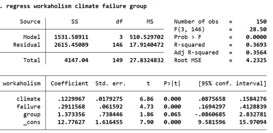
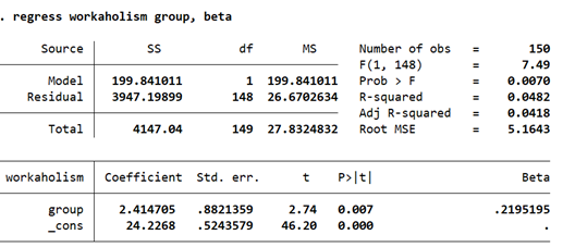
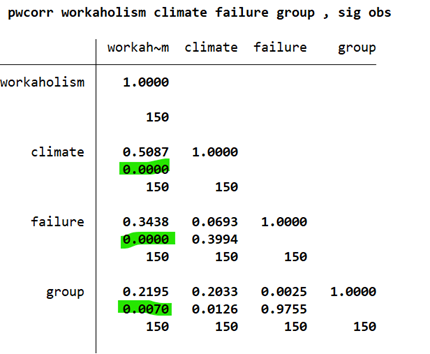
regress workaholicm climate failure group Source SS df MS Number of obs 150 F(3, 146) 28.50 Model 1531. 58911 3 510.529702 Prob > F E 0.0900 Residual 2615. 45089 146 17.9140472 R-squared 0.3693 Adj R-squared 0.3564 Total 4147.04 149 27.8324832 Root MSE 4.2325 workaholis Coefficient Std. err. t P>It| [95% conf. interval] climate . 1229967 . 0179275 6.86 9.090 . 0875658 . 1584276 failure . 2911568 . 061592 4.73 0.090 . 1694297 . 4128839 group 1.373356 . 738446 1.86 0.065 - . 0860685 2.832781 _cons 12.77627 1. 616455 7.90 0.090 9.581596 15.97094regress workaholicm group, beta Source SS df MS Number of obs 150 ii F (1, 148) 7.49 Model 199. 841011 1 199. 841011 Prob > F 0. 0970 Residual 3947 . 19899 148 26.6702634 R-squared 0. 0482 Adj R-squared 0. 0418 Total 4147.04 149 27.8324832 Root MSE 5.1643 workaholicm Coefficient Std. err. t P> /t| Beta group 2.414705 . 8821359 2.74 0.007 . 2195195 cons 24.2268 . 5243579 46. 20 6.090pwcorr workaholicm climate failure group , sig obs workah~m climate failure group workaholis 1.0909 150 climate 0. 5087 1.0000 0.0000 150 150 failure 0.3438 0.0693 1.0900 0.0000 0. 3994 150 150 150 group 0.2195 0. 2033 0. 0025 1.0900 0.0070 0. 0126 0.9755 150 150 150 150