I am stumped and need help desperately!

attached is the problem I am stuck on.

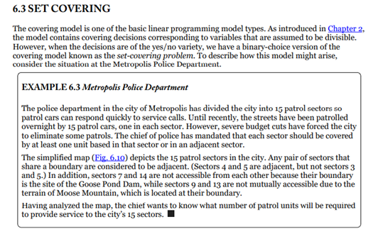
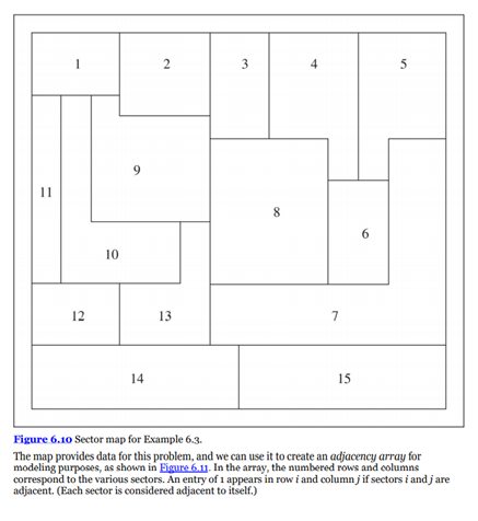
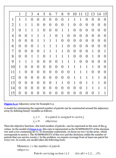
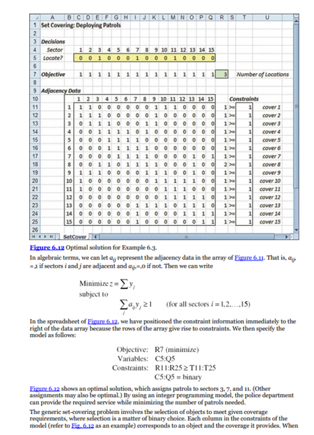
6.3 SET COVERING The covering model is one of the basic linear programming model types. As introduced in Chapter 2, the model contains covering decisions corresponding to variables that are assumed to be divisible. However, when the decisions are of the yeso variety, we have a binary-choice version of the covering model known as the set-covering problem. To describe how this model might arise, consider the situation at the Metropolis Police Department. EXAMPLE 6.3 Metropolis Police Department The police department in the city of Metropolis has divided the city into 15 patrol sectors so patrol cars can respond quickly to service calls. Until recently, the streets have been patrolled overnight by 15 patrol cars, one in each sector. However, severe budget cuts have forced the city to eliminate some patrols. The chief of police has mandated that each sector should be covered by at least one unit based in that sector or in an adjacent sector. The simplified map (Fig. 6.10) depicts the 15 patrol sectors in the city. Any pair of sectors that share a boundary are considered to be adjacent. (Sectors 4 and 5 are adjacent, but not sectors 3 and 5.) In addition, sectors 7 and 14 are not accessible from each other because their boundary is the site of the Goose Pond Dam, while sectors 9 and 13 are not mutually accessible due to the terrain of Moose Mountain, which is located at their boundary. Having analyzed the map, the chief wants to know what number of patrol units will be required to provide service to the city's 15 sectors. 2 2 3 4 5 9 11 8 6 10 12 13 7 14 15 Figure 6.10 Sector map for Example 6.3. The map provides data for this problem, and we can use it to create an adjacency array for modeling purposes, as shown in Figure 6.11. In the array, the numbered rows and columns correspond to the various sectors. An entry of 1 appears in row i and column jif sectors i and jare adjacent. (Each sector is considered adjacent to itself.) 2 1 2 3 4 5 6 7 8 9 10 11 12 13 14 15 1 1 1 0 0 0 0 0 0 1 1 1 0 0 0 0 2 1 1 1 0 0 0 0 0 1 0 0 0 0 0 0 3 0 1 1 1 0 0 0 1 1 0 0 0 0 0 0 4 0 0 1 1 1 10 1 0 0 0 0 0 0 0 5 0 0 0 1 1 1 1 0 0 0 0 0 0 0 0 6 0 0 011 1 1 1 0 0 0 0 0 0 0 7 0 0 0 0 1 1 1 1 0 0 0 0 1 0 1 8 0 0 1 1 01111 0 0 0 1 0 0 9 1 1 1 0 0 0 0 1 1 1 0 0 0 0 0 10 1 0 0 0 0 0 0 0 1 1 1 1 1 0 0 11 1 0 0 0 0 0 0 0 0 1 1 1 0 0 0 12 0 0 0 0 0 0 0 0 0 1 1 1 1 1 0 13 0 0 0 0 0 0 1 1 0 1 0 1 1 1 0 14 0 0 0 0 0 0 0 0 0 0 0 1 1 1 1 15 0 0 0 0 0 0 0 0 0 0 0 0 0 1 1 Figure 6.11 Adjacency array for Example 63. A model for minimizing the required number of patrols can be constructed around the adjacency array by defining binary variables as follows: if a patrol is assigned to sector y = 0 otherwise Then the objective function-the total number of patrols-can be expressed as the sum of the values. In the model of Figure 6.12. this sum is represented as the SUMPRODUCT of the decision row and a row containing all i's. To formulate constraints, we focus on row in the array, which corresponds to sector i. The SUMPRODUCT of this row and the decisions yields the number of patrols that can service county i. In the problem, we require coverage from at least one patrol for every row. In words, our model takes the following form: Minimize z = the number of patrols subject to Patrols servicing section / 21 (for all i = 1.2.....15) T BCDEFGHI K L M N O PO RS U 1 Set Covering: Deploying Patrols 2 3 Decisions 4 Sector 1 2 3 4 5 6 7 8 9 10 11 12 13 14 15 5 Locate? 00100010001000 6 7 Objective Number of Locations 8 9 Adjacency Data 10 1 2 3 4 5 6 7 8 9 10 11 12 13 14 15 Constraints 11 1 1 1 0 0 0 0 0 0 1 1 1 0 0 0 0 1 cover 1 12 2 1 1 1 0 0000 1000000 1 > 1 cover 2 13 301 11000 11000000 1 cover 3 14 400 1111010OOOOOO 1 1 cover a 15 50001 11100OOOOOO 1 > 1 covers 16 600011 1110000000 1 > 1 cover 6 17 7000011110000101 1 > 1 cover 7 18 8001101111000100 2 1 cover 8 19 9 1 1 0 0 0 0 1 1 1 0 0 1 0 0 1 cover 20 10 10 OOOOOO 1 1 1 1 1 0 0 1 1 cover 10 21 11 1000000001 1 1 1 0 0 0 1 > 1 cover 11 22 1 cover 12 23 13 O OOOOO 1 1 1 1 0 1 1 1 0 1 cover 10 24 14 0 0 0 0 0 0 1 0 0 0 0 1 1 1 1 1 cover 14 25 15 OOOOOOOOOOO011 1 > 1 cover 15 26 HMI Set Cover Figure 6.12 Optimal solution for Example 6-3. In algebraic terms, we can let a represent the adjacency data in the array of Figure 6.11. That is, ay = 1 if sectors i and jare adjacent and ayo if not. Then we can write Minimize z=y subject to Say, 21 (for all sectors i = 1,2...15) In the spreadsheet of Figure 6.12. we have positioned the constraint information immediately to the right of the data array because the rows of the array give rise to constraints. We then specify the model as follows: Objective: R7 (minimize) Variables: C5:25 Constraints: R11:R252T11:T25 C5:05 = binary Eigure 6.12 shows an optimal solution, which assigns patrols to sectors 3.7 and 11. (Other assignments may also be optimal.) By using an integer programming model, the police department can provide the required service while minimizing the number of patrols needed The generic set-covering problem involves the selection of objects to meet given coverage requirements, where selection is a matter of binary choice. Each column in the constraints of the model (refer to Fig.6.12 as an example) corresponds to an object and the coverage it provides. When the coverage is expressed with o's and 1's (the constraint coefficients in a column), we can think of the 1's as defining a coverage set (i.e., the set of rows in which i's appear). Thus, the selection of objects is equivalent to the selection of sets, and the problem is to choose the minimum number of sets that will provide the required coverage. This interpretation gives rise to the name set-covering problem. 6.3 SET COVERING The covering model is one of the basic linear programming model types. As introduced in Chapter 2, the model contains covering decisions corresponding to variables that are assumed to be divisible. However, when the decisions are of the yeso variety, we have a binary-choice version of the covering model known as the set-covering problem. To describe how this model might arise, consider the situation at the Metropolis Police Department. EXAMPLE 6.3 Metropolis Police Department The police department in the city of Metropolis has divided the city into 15 patrol sectors so patrol cars can respond quickly to service calls. Until recently, the streets have been patrolled overnight by 15 patrol cars, one in each sector. However, severe budget cuts have forced the city to eliminate some patrols. The chief of police has mandated that each sector should be covered by at least one unit based in that sector or in an adjacent sector. The simplified map (Fig. 6.10) depicts the 15 patrol sectors in the city. Any pair of sectors that share a boundary are considered to be adjacent. (Sectors 4 and 5 are adjacent, but not sectors 3 and 5.) In addition, sectors 7 and 14 are not accessible from each other because their boundary is the site of the Goose Pond Dam, while sectors 9 and 13 are not mutually accessible due to the terrain of Moose Mountain, which is located at their boundary. Having analyzed the map, the chief wants to know what number of patrol units will be required to provide service to the city's 15 sectors. 2 2 3 4 5 9 11 8 6 10 12 13 7 14 15 Figure 6.10 Sector map for Example 6.3. The map provides data for this problem, and we can use it to create an adjacency array for modeling purposes, as shown in Figure 6.11. In the array, the numbered rows and columns correspond to the various sectors. An entry of 1 appears in row i and column jif sectors i and jare adjacent. (Each sector is considered adjacent to itself.) 2 1 2 3 4 5 6 7 8 9 10 11 12 13 14 15 1 1 1 0 0 0 0 0 0 1 1 1 0 0 0 0 2 1 1 1 0 0 0 0 0 1 0 0 0 0 0 0 3 0 1 1 1 0 0 0 1 1 0 0 0 0 0 0 4 0 0 1 1 1 10 1 0 0 0 0 0 0 0 5 0 0 0 1 1 1 1 0 0 0 0 0 0 0 0 6 0 0 011 1 1 1 0 0 0 0 0 0 0 7 0 0 0 0 1 1 1 1 0 0 0 0 1 0 1 8 0 0 1 1 01111 0 0 0 1 0 0 9 1 1 1 0 0 0 0 1 1 1 0 0 0 0 0 10 1 0 0 0 0 0 0 0 1 1 1 1 1 0 0 11 1 0 0 0 0 0 0 0 0 1 1 1 0 0 0 12 0 0 0 0 0 0 0 0 0 1 1 1 1 1 0 13 0 0 0 0 0 0 1 1 0 1 0 1 1 1 0 14 0 0 0 0 0 0 0 0 0 0 0 1 1 1 1 15 0 0 0 0 0 0 0 0 0 0 0 0 0 1 1 Figure 6.11 Adjacency array for Example 63. A model for minimizing the required number of patrols can be constructed around the adjacency array by defining binary variables as follows: if a patrol is assigned to sector y = 0 otherwise Then the objective function-the total number of patrols-can be expressed as the sum of the values. In the model of Figure 6.12. this sum is represented as the SUMPRODUCT of the decision row and a row containing all i's. To formulate constraints, we focus on row in the array, which corresponds to sector i. The SUMPRODUCT of this row and the decisions yields the number of patrols that can service county i. In the problem, we require coverage from at least one patrol for every row. In words, our model takes the following form: Minimize z = the number of patrols subject to Patrols servicing section / 21 (for all i = 1.2.....15) T BCDEFGHI K L M N O PO RS U 1 Set Covering: Deploying Patrols 2 3 Decisions 4 Sector 1 2 3 4 5 6 7 8 9 10 11 12 13 14 15 5 Locate? 00100010001000 6 7 Objective Number of Locations 8 9 Adjacency Data 10 1 2 3 4 5 6 7 8 9 10 11 12 13 14 15 Constraints 11 1 1 1 0 0 0 0 0 0 1 1 1 0 0 0 0 1 cover 1 12 2 1 1 1 0 0000 1000000 1 > 1 cover 2 13 301 11000 11000000 1 cover 3 14 400 1111010OOOOOO 1 1 cover a 15 50001 11100OOOOOO 1 > 1 covers 16 600011 1110000000 1 > 1 cover 6 17 7000011110000101 1 > 1 cover 7 18 8001101111000100 2 1 cover 8 19 9 1 1 0 0 0 0 1 1 1 0 0 1 0 0 1 cover 20 10 10 OOOOOO 1 1 1 1 1 0 0 1 1 cover 10 21 11 1000000001 1 1 1 0 0 0 1 > 1 cover 11 22 1 cover 12 23 13 O OOOOO 1 1 1 1 0 1 1 1 0 1 cover 10 24 14 0 0 0 0 0 0 1 0 0 0 0 1 1 1 1 1 cover 14 25 15 OOOOOOOOOOO011 1 > 1 cover 15 26 HMI Set Cover Figure 6.12 Optimal solution for Example 6-3. In algebraic terms, we can let a represent the adjacency data in the array of Figure 6.11. That is, ay = 1 if sectors i and jare adjacent and ayo if not. Then we can write Minimize z=y subject to Say, 21 (for all sectors i = 1,2...15) In the spreadsheet of Figure 6.12. we have positioned the constraint information immediately to the right of the data array because the rows of the array give rise to constraints. We then specify the model as follows: Objective: R7 (minimize) Variables: C5:25 Constraints: R11:R252T11:T25 C5:05 = binary Eigure 6.12 shows an optimal solution, which assigns patrols to sectors 3.7 and 11. (Other assignments may also be optimal.) By using an integer programming model, the police department can provide the required service while minimizing the number of patrols needed The generic set-covering problem involves the selection of objects to meet given coverage requirements, where selection is a matter of binary choice. Each column in the constraints of the model (refer to Fig.6.12 as an example) corresponds to an object and the coverage it provides. When the coverage is expressed with o's and 1's (the constraint coefficients in a column), we can think of the 1's as defining a coverage set (i.e., the set of rows in which i's appear). Thus, the selection of objects is equivalent to the selection of sets, and the problem is to choose the minimum number of sets that will provide the required coverage. This interpretation gives rise to the name set-covering