i) Begin by looking at the relationship between each product and its own price. For both products separately, do/answer the following:

a. First, make the scatter plot of price (on the vertical axis) and quantity sold (on the horizontal axis). Insert a trend line into each graph and display the equation of the line. This is a crude measure of the inverse demand curve. From the equation of the trendline, fill in the equation of the inverse demand curve for each good in the box below.

Insert separate graphs for each good here:

Regular (good 1): Inverse demand equation: P1 = _________ - _________ Q1

Organic (good 2): Inverse demand equation: P2 = _________ - _________ Q2

c. Is there a negative relationship between quantity sold and the product's price? Provide an economic (or managerial) interpretation of the slope of these lines. (ie., what do these specific numbers mean?)

We are now interested in estimating the demand function, with Quantity (Q) as the dependent variable and price (P) as the explanatory variable (as opposed to the inverse demand function, with P as the dependent variable and Q as the explanatory variable, graphed above). We know that demand for a product is not only influenced by its price, but also the price of the other product, among other variables. So instead of just graphing the relationship between Q and P, similar to what we did above, we will use Excel's Regression tool, as this will allow us to control for other variables. (See section 3.2 in the textbook for an example of using this tool to estimate a simple inverse demand curve. See also the example "Example Demand Estimation" file in folder Unit 1F). We will use the results from the regressions to answer several questions.

For each good, do/answer the following (d-l):

d. Carry out a multiple regression using linear specification, with quantity as the dependent (left-hand side, or y) variable and own price, other good's price, income, and temperature as explanatory (right-hand side or x) variables. Because you are including more than one variable as explanatory variables, you will need to highlight all the cells of explanatory variables when you indicate the X-range using the regression tool. I recommend having the columns for each explanatory variable right next to each other in the spreadsheet for this purpose.

Insert the regression output for each good here:

e. What are your estimated demand equations for each good (ie., Q as a function of all the variables you included in the regression, including the intercept)?,

Regular (good 1): Inverse demand equation: P1 = _________ - _________ Q1

Organic (good 2): Inverse demand equation: P2 = _________ - _________ Q2d.

f. What are the R-squared statistics from each regression? For which product does the demand function explain more of the variation in sales?

g. Let's now focus on the effect of a good's own price. What is the coefficient estimate for that same good's price? Provide an economic interpretation of those numbers (eg., by how much does quantity vary with a change in price)? Given the standard errors or the p-values given in the regressions, are these coefficient estimates statistically significant at the 5% significance level?

h. We are interested in how responsive consumers are to changes in price for each good. To quantify their responsiveness, calculate the price elasticity of demand for each product using the regression estimates from part d (see equation 3.6 or refer to Q&A 3.2 in the textbook). As you know, elasticity will vary along the linear demand curve, so you'll need to pick a point at which to calculate the elasticities. Choose the product's average Q and average P in the dataset. Interpret these elasticities (ie., quantitatively, what do these particular numbers mean?). Is demand for either product elastic or inelastic?

Regular (good 1):

Average P1 in data set =

Average Q1 in data set =

Elasticity (?1) =

Interpretation of elasticity:

Organic (good 2):

Average P2 in data set =

Average Q2 in data set =

Elasticity (?2) =

Interpretation of elasticity:

i. Based on the elasticities from part h, is demand for either product "elastic" or "inelastic"? The owners of iScream are interested in knowing what would happen to revenue from their original ice cream cones if they increase its price slightly from the average price of the good in the data (holding everything else constant). Based on the estimated elasticity, would revenue increase, decrease, or stay about the same? Similarly, they are interested in knowing how revenue from their organic product would change if they were to increase its price slightly from the average (holding everything else constant). Would revenue increase, decrease, or stay about the same?

j. Let's now look at the effects of some of the other variables in the demand equation. What is the effect of consumer average income on sales? Are the goods normal or inferior goods? (No calculations needed.)

k. How is demand for one good affected by the price of the other good? Which good is more affected by the price of the other good? Are the goods substitutes or complements? (No calculations needed.)

l. The summer is fast approaching, and experts are disagreeing over how hot the summer is going to be. Some are forecasting an unusually hot summer, with average high temperatures predicted to reach 90 degrees in July. Others are predicting an unusually cool summer, with an average high temperature in July of only 78. The owners of iScream would like to know how this difference in possible temperatures will affect their sales. At the averages in the dataset of all other variables, use the regression equations (part e) to predict the number of units sold in a month of each good under two scenarios: i) the monthly high averages 90 degrees; ii) the monthly high averages 78 degrees. Note that because the data are in monthly sales by region (of which there are 8), you'll need to multiply the number of units predicted from the regression equation by 8 in order to get total predicted units sold in a month.

Predicted monthly sales: Regular (Q1) /Organic (Q2)

78 degrees/ ____________/________________

90 degree/______________/_________________

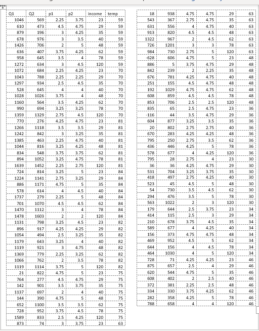
The data is attached below and is read continuously as if the left 6 columns are stacked on top of the right 6 columns. Any help or information at all would be extremely helpful! Seriously, if just any part of this could be explained or answered it would help me out so much! I have never taken this type of class before and I am struggling to catch up.

Q1 02 income itemp 18 9013 4.7! 4.75 29 1046 569 2.25 3.75 59 543 49E 2.75 1.75 35 63 610 473 1.5 4.75 29 59 601 556 4.75 40 63 179 196 4.25 35 913 4.5 4.5 48 1 63 678 976 31 40 1322 967 4.5 1426 706 2 1 50 726 1201 78 63 636 407 3.75 62 591 984 730 2.75 5 120 63 645 3.5 78 59 1 628 606 4.7 5 23 48 1272 634 4.3 120 59 186 5 3.75 1.75 29 48 1072 684 4.25 23 70 #42 239 2 2.25 35 48 1043 788 2.25 1 2.25 29 70 676 781 1.25 4.75 40 1297 934 2.5 4.5 70 1 251 155 4.5 4.75 48 48 528 645 4 40 70 192 1029 4.75 4.75 62 1028 48 1026 3.75 4 48 70 1 859 4.5 4.5 48 1160 564 3.5 4.25 62 70 1 853 706 2.5 2.5 120 48 990 :94 3.25 3.25 78 70 135 65 2.5 4.75 23 1359 1329 2.75 4.5 120 70 116 44 3.5 4.75 29 36: 770 276 4.25 1.75 23 81 ; 604 177 3.25 3.5 35 36 1266 1118 3.5 1 4.5 291 81 1 20 802 2.75 2.75 1242 842 40 36 3.25 35 81 1 670 283 4.25 4.25 48 36 1385 463 2.25 4.75 40 795 250 2.75 3.5 62 36 1044 3.25 4.25 81 1 436 446 4.25 36 1 834 548 3.75 3.75 62 81 : 578 677 1 4.25 120 894 1052 36 3.25 4.75 81 1 795 2.75 23 30 1639 1452 2.25 2.75 120 81 ; 36 4.25 29 724 814 30 3.25 5 1 84 1 531 704 3.25 3.75 35 30 1224 1141 2.75 3.25 29 84 1 418 497 2.75 4.25 40 30 186 1171 4.75 5 35 84 1 523 45 4.5 5 : 48 30 578 614 4 1 4.5 40 84 1 54 730 3.5 4.5 62 30 1737 279 2.25 84 1 294 476 3.5 78 30 701 1070 4.5 4.5 62 84 1 563 1022 2 1 120 1470 1112 31 78 84 1 179 644 2.5 23 1478 1603 2 120 84 1 414 115 29 1131 798 3.25 4.5 23 82 1 210 --- 678 3.75 34 896 917 4.25 4.25 29 82 1 589 677 4 4.25 40 34 1054 194 2.5 3.25 35 82 156 373 4.75 4.75 34 1179 643 3.25 4 1 40 82 469 952 1.5 62 1119 921 4.75 48 82 1 644 156 4 1.5 34 59ET 779 2.25 3.25 62_1 82 464 1030 120 34 1066 762 2 3.5 78 82 728 714 4.25 .25 46 1119 1114 3.75 5 120 82 875 657 2.5 4 --+- 46 21 822 4.75 Hun i 23 75 1 620 544 4.75 i un i 35 46 764 277 4.5 4.75 29 75 : 402 2.5 40 46 142 901 3.5 3.75 35 172 381 2.25 2.5 46 1137 697 _21 40 134 330 3.75 62 46 144 390 4.75 48 75 282 358 4.25 78 46 652 1100 3.5 3.5 62 75 788 6SE 120 46 728 952 3.75 4.5 78 75 1589 833 2.5 4.25 120 75 1 74 3.75 23 63