I need a little help for my projecte. Objective: Comparative study of Dimensionality Reduction Techniques and their Impact on

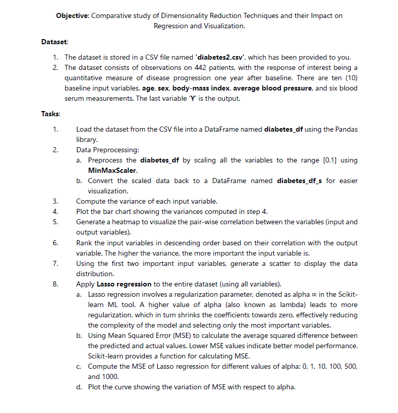
Regression and Visualization.

Dataset:

The dataset is stored in a CSV file named 'diabetes$2.$csv$\text{'},$ which has been provided to you.

The dataset consists of observations on $442$ patients, with the response of interest being a

quantitative measure of disease progression one year after baseline. There are ten $(10)$

baseline input variables, age, sex, body$-$mass index, average blood pressure, and six blood

serum measurements. The last variable $\text{'}Y\text{'}$ is the output.

Task:

Load the dataset from the CSV file into a DataFrame named diabetes$\_$df using the Pandas

library.

Data Preprocessing:

a$.$ Preprocess the diabetes$\_$df by scaling all the variables to the range $0,1$ using

MinMaxScaler.

b$.$ Convert the scaled data back to a DataFrame named diabetes$\_$df$\_$s for easier

visualization.

Compute the variance of each input variable.

Plot the bar chart showing the variances computed in step $4.$

Generate a heatmap to visualize the pair$-$wise correlation between the variables $($input and

output variables$).$

Rank the input variables in descending order based on their correlation with the output

variable. The higher the variance, the more important the input variable is$.$

Using the first two important input variables, generate a scatter to display the data

distribution.

Apply Lasso regression to the entire dataset $($using all variables$).$

a$.$ Lasso regression involves a regularization parameter, denoted as alpha prop in the Scikit$-$

learn ML tool. A higher value of alpha $($also known as lambda$)$ leads to more

regularization, which in turn shrinks the coefficients towards zero, effectively reducing

the complexity of the model and selecting only the most important variables.

b$.$ Using Mean Squared Error $($MSE$)$ to calculate the average squared difference between

the predicted and actual values. Lower MSE values indicate better model performance.

Scikit$-$learn provides a function for calculating MSE.

c$.$ Compute the MSE of Lasso regression for different values of alpha: $0,1,10,100,500,$

and $1000.$

d$.$ Plot the curve showing the variation of MSE with respect to alpha.

Display the best MSE and the corresponding alpha value.

f$.$ Plot the evolution of Lasso coefficients against alpha to observe how they change and

how they are Shrunk as alpha varies.

Reduce the data dimensionality using PCA $($Principal Component Analysis$).$

a$.$ Utilize PC$1$ and PC$2$ and visualize the data scatter.

b$.$ Plot the loadings to examine how the variables contribute to PC$1$ and PC$2.$

c$.$ Perform normal linear regression, using PC$1$ only.

d$.$ Plot the regression line on the scatter.

e$.$ Perform normal linear regression, using PC$1$ and PC$2.$

f$.$ Plot the regression hyper$-$line on the scatter.

g$.$ Using bar chart, calculate, and display the MSE for both cases $9.$c and $9.$d$.$

Reduce the data dimensionality with t$-$SNE.

a$.$ Utilize the $1$st and $2$nd t$-$SNE dimensions to visualize the data scatter, with different

perplexity values: $5,10,20,$ and $50.$

b$.$ Perform normal linear regression, using only the $1^($st $)$ dimension of t$-$SNE.

c$.$ Plot the regression line on the scatter.

d$.$ Perform normal linear regression, using the $1^($st $)$ and $2^($nd $)$ dimensions of t$-$SNE.

e$.$ Plot the regression hyper$-$line on the scatter.

f$.$ Using bar chart, calculate, and display the MSE for both cases $10.$b and $10.$d$.$

Reduce the data dimensionality with UMAP.

a$.$ Utilize the $1$st and $2$nd UMAP dimensions to visualize the data scatter, with different

n$\_$neighbors $($number of neighbors$)$ values: $5,10,20,$ and $50.$

b$.$ Perform normal linear regression, using only the $1^($st $)$ dimension of UMAP.

c$.$ Plot the regression line on the scatter.

d$.$ Perform normal linear regression, using the $1^($st $)$ and $2^($nd $)$ dimensions of UMAP.

e$.$ Plot the regression hyper$-$line on the scatter.

f$.$ Using bar chart, calculate, and display the MSE for both cases $11.$b and $11.$d$.$

g$.$ Provide a comparative table to compare Linear Regression applied to PCA, t$-$SNE, and

UMAP data, utilizing the first three dimensions for each dimensionality reduction

method.

Objective: Comparative study of Dimensionality Reduction Techniques and their Impact on

Regression and Visualization.

Dataset:

The dataset is stored in a CSV file named 'diabetes$2.$csv$\text{'},$ which has been provided to you.

The dataset consists of observations on $442$ patients, with the response of interest being a

quantitative measure of disease progression one year after baseline. There are ten $(10)$

baseline input variables, age, sex, body$-$mass index, average blood pressure, and six blood

serum measurements. The last variable $\text{'}$ Y $\text{'}$ is the output.

Task:

Load the dataset from the CSV file into a DataFrame named diabetes$\_$df using the Pandas

library.

Data Preprocessing:

a$.$ Preprocess the diabetes$\_$df by scaling all the variables to the range $0,1$ using

MinMaxScaler.