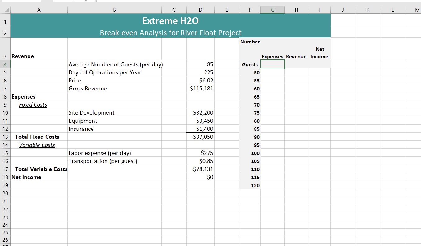
I need help figuring out how to complete these last step on the Excel. I don't know how to make a data table with conditional formating with this data. I need to know what to put in the Data Table when it says "row imput cell" and column input cell and I also need help with the rest of the steps to complete this assignment.

Instructions:

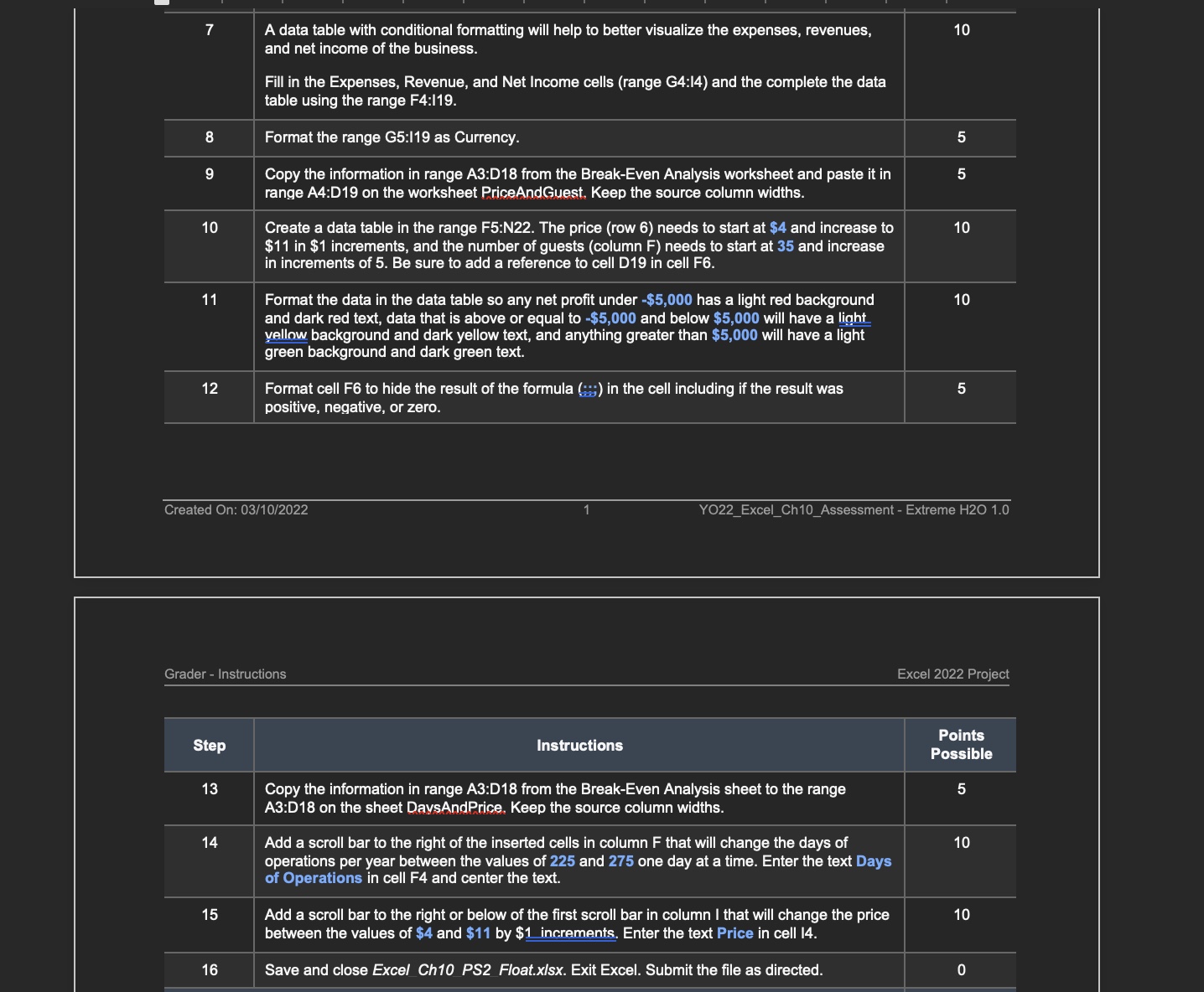
Extreme H2O \begin{tabular}{|c|c|c|} \hline 7 & \begin{tabular}{l} A data table with conditional formatting will help to better visualize the expenses, revenues, \\ and net income of the business. \\ Fill in the Expenses, Revenue, and Net Income cells (range G4:14) and the complete the data \\ table using the range F4:I19. \end{tabular} & 10 \\ \hline 8 & Format the range G5:I19 as Currency. & 5 \\ \hline 9 & \begin{tabular}{l} Copy the information in range A3:D18 from the Break-Even Analysis worksheet and paste it in \\ range A4:D19 on the worksheet PriceAndGuest. Keep the source column widths. \end{tabular} & 5 \\ \hline 10 & \begin{tabular}{l} Create a data table in the range F5:N22. The price (row 6 ) needs to start at $4 and increase to \\ $11 in $1 increments, and the number of guests (column F) needs to start at 35 and increase \\ in increments of 5 . Be sure to add a reference to cell D19 in cell F6. \end{tabular} & 10 \\ \hline 11 & \begin{tabular}{l} Format the data in the data table so any net profit under $5,000 has a light red background \\ and dark red text, data that is above or equal to $5,000 and below $5,000 will have a light \\ vellow background and dark yellow text, and anything greater than $5,000 will have a light \\ green background and dark green text. \end{tabular} & 10 \\ \hline 12 & \begin{tabular}{l} Format cell F6 to hide the result of the formula (:.3) in the cell including if the result was \\ positive, negative, or zero. \end{tabular} & 5 \\ \hline \multicolumn{2}{|c|}{ Created On: 03/10/2022 } & eH2O1.0 \\ \hline \end{tabular} Grader - Instructions Excel 2022 Project \begin{tabular}{c|l|c} \hline Step & \multicolumn{1}{|c}{ Instructions } & \begin{tabular}{c} Points \\ Possible \end{tabular} \\ \hline 13 & \begin{tabular}{l} Copy the information in range A3:D18 from the Break-Even Analysis sheet to the range \\ A3:D18 on the sheet DaysAndPrice. Keep the source column widths. \end{tabular} & 5 \\ \hline 14 & \begin{tabular}{l} Add a scroll bar to the right of the inserted cells in column F that will change the days of \\ operations per year between the values of 225 and 275 one day at a time. Enter the text Days \\ of Operations in cell F4 and center the text. \end{tabular} & 10 \\ \hline 15 & \begin{tabular}{l} Add a scroll bar to the right or below of the first scroll bar in column I that will change the price \\ between the values of $4 and $11 by $1 increments. Enter the text Price in cell 14. \end{tabular} & 10 \\ \hline 16 & Save and close Excel Ch10 PS2 Float.x/sx. Exit Excel. Submit the file as directed. & 0 \\ \hline \end{tabular}