i need help follwing the steps and putting in the formulas right on excel

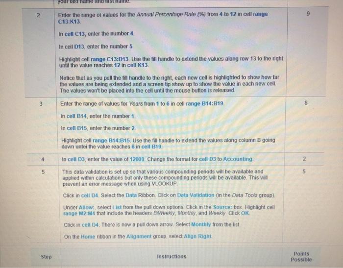
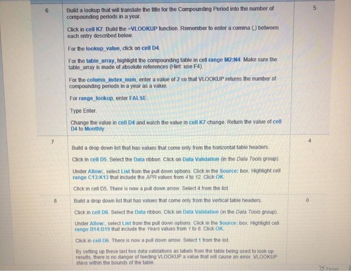
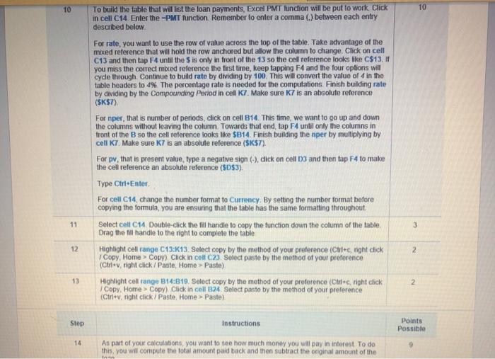
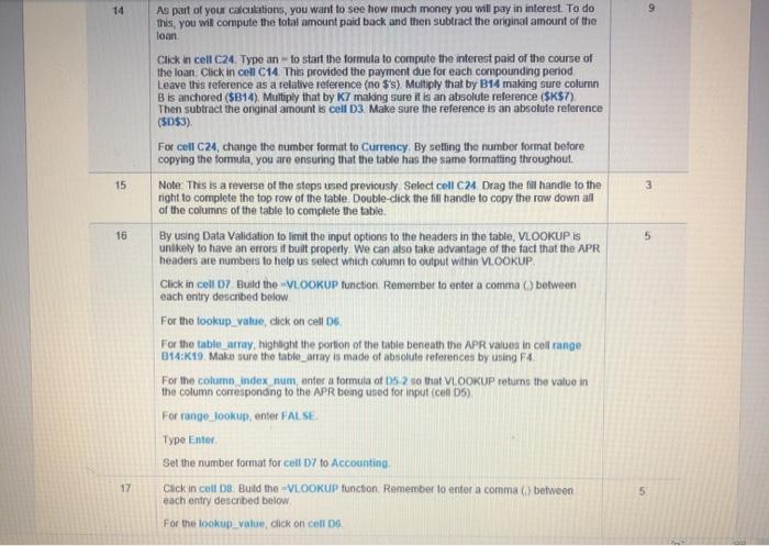
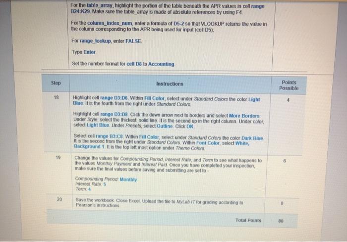
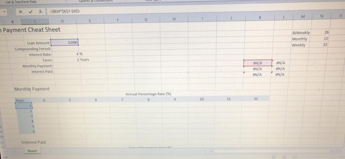
10 10 To build the table that will list the loan payments, Excel PMT function will be put to work Click in cell C14 Enter the PMT function. Remember to enter a comma () between each entry described below For rate, you want to use the row of value across the top of the table. Take advantage of the mixed reference that will hold the row anchored but allow the column to change. Click on cell C13 and then tap F4 until the S is only in front of the 13 so the cell reference looks like C$13, 11 you miss the correct med reference the first time, keep tapping F4 and the four options will cycle through. Continue to build rate by dividing by 100. This will convert the value of 4 in the table headers to 4% The percentage rate is needed for the computations. Finish building rate by dividing by the Compouncting Period in cell 7. Make sure K7 is an absolute reference ($K$7) For nper, that is number of periods, click on cell B14. This time, we want to go up and down the columns without leaving the column. Towards that end, tap F4 until only the colurins in front of the B so the cell reference looks like $B14 Finish building the nper by multiplying by cell K7. Make sure K7 is an absolute reference ($K$7). For pv that is present value, type a negative sign (-), click on cell 13 and then tap F4 to make the cell reference an absolute reference ($D$3). Type Ctri Enter Forcell C14, change the number format to Currency. By setting the number format before copying the formula, you are ensuring that the table has the same formatting throughout Select cell C14 Double-click the fill handle to copy the function down the column of the table Drag the handle to the right to complete the table Highlight cell range C13:K13. Select copy by the method of your preference (Ctrl+c night click Copy, Home > Copy). Click in cell C23 Select paste by the method of your preference (Ctrl+v, right click / Paste, Home > Paste) Highlight cel rango B14:B19. Select copy by the method of your preference (Crec right click Copy. Home Copy) Click in cell B24 Select paste by the method of your preference (Ctrl+v, right click / Paste, Home > Paste) 11 3 12 2 13 2 Step Instructions Points Possible 14 As part of your calculations, you want to see how much money you will pay in interest to do this, you will compute the lotal amount paid back and then subtract the original amount of the 14 9 As part of your calculations, you want to see how much money you will pay in interest. To do this, you will compute the total amount paid back and then subtract the original amount of the loan 15 3 16 5 Click in cell C24. Type an-to start the formula to compute the interest paid of the course of the loan Click in cell C14. This provided the payment due for each compounding period Leave this reference as a relative reference (no $s) Multiply that by B14 making sure column Bis anchored ($B14). Multiply that by Ky making sure it is an absolute reference ($K$7) Then subtract the onginal amount is cell D3. Make sure the reference is an absolute reference ($D$3) For cell C24, change the number format to Currency. By selling the number format before copying the formula, you are ensuring that the table has the same formatting throughout Note: This is a reverse of the steps used previously Select cell C24 Drag the fill handle to the right to complete the top row of the table Double-click the fill handle to copy the row down all of the columns of the table to complete the table. By using Data Validation to limit the input options to the headers in the table, VLOOKUP is unlikely to have an errors if built properly. We can also take advantage of the fact that the APR headers are numbers to help us select which column to output within VLOOKUP Click in cell 07 Build the VLOOKUP function. Remember to enter a comma (between each entry described below For the lookup_value, click on cell 16 For the table array, highlight the portion of the table beneath the APR values in col range B14:K19 Make sure the table_arrays made of absolute references by using F4 For the column_index_num enter a formula of D5 2 so that VLOOKUP returns tho value in the column corresponding to the APR being used for input (cello) For range_lookup, enter FALSE Type Enter Set the number format for cell D7 to Accounting Click in cell D. Build the VLOOKUP function Remember to enter a comma () between each entry described below For the lookup_value dick on cells 17 5 For the table array, highlight the portion of the table beneath the APR values in cell range B24:K29. Make sure the table_array is made of absoluto references by using F4. For the column_index_num, enter a formula of 05-2 so that VLOOKUP returns the value in the column corresponding to the APR being used for input (cel 05). For range_lookup, enter FALSE Type Enter Set the number format for cell be to Accounting Step Instructions Points Possible 18 4 Highlight coll range 03:06. Within Fill Color, select under Standard Colors the color Light Blue It is the fourth from the right under Standard Colors Highlight cell range 03:08 Click the down arrow next to borders and select More Borders Under Style, select the thickest, solid line. It is the second up in the right column. Under color select Light Blue Under Presets, select Outline. Click OK Select coll range 33:C8. Within Fill Color, select under Standard Colors the color Dark Blue It is the second from the right under Standard Colors. Within Font Color, select White Background 1 It is the top left most option under Theme Colors Change the values for Compounding Period, Interest Rate, and Term to see what happens to the values Monthly Payment and interest Paid Once you have completed your inspection make sure the final values before saving and submitting are set to Compounding Period Monthly Interest Rate 5 Term. 4 Save the workbook Close Excent. Upload the file to MyLab IT for grading according to Pearson's instruction 19 6 20 0 Total Points De Com -5814557-5853 M N G H D Payment Cheat Sheet BrWeekly Monthly Weekly 26 12 52 1 an Amount Compounding Patio Interest rate: Term Montent Interestad 1 Years N/A N/A MA N/A MN/A N/A Monthly Payment Manual Percentage 10 interest Paid 10 10 To build the table that will list the loan payments, Excel PMT function will be put to work Click in cell C14 Enter the PMT function. Remember to enter a comma () between each entry described below For rate, you want to use the row of value across the top of the table. Take advantage of the mixed reference that will hold the row anchored but allow the column to change. Click on cell C13 and then tap F4 until the S is only in front of the 13 so the cell reference looks like C$13, 11 you miss the correct med reference the first time, keep tapping F4 and the four options will cycle through. Continue to build rate by dividing by 100. This will convert the value of 4 in the table headers to 4% The percentage rate is needed for the computations. Finish building rate by dividing by the Compouncting Period in cell 7. Make sure K7 is an absolute reference ($K$7) For nper, that is number of periods, click on cell B14. This time, we want to go up and down the columns without leaving the column. Towards that end, tap F4 until only the colurins in front of the B so the cell reference looks like $B14 Finish building the nper by multiplying by cell K7. Make sure K7 is an absolute reference ($K$7). For pv that is present value, type a negative sign (-), click on cell 13 and then tap F4 to make the cell reference an absolute reference ($D$3). Type Ctri Enter Forcell C14, change the number format to Currency. By setting the number format before copying the formula, you are ensuring that the table has the same formatting throughout Select cell C14 Double-click the fill handle to copy the function down the column of the table Drag the handle to the right to complete the table Highlight cell range C13:K13. Select copy by the method of your preference (Ctrl+c night click Copy, Home > Copy). Click in cell C23 Select paste by the method of your preference (Ctrl+v, right click / Paste, Home > Paste) Highlight cel rango B14:B19. Select copy by the method of your preference (Crec right click Copy. Home Copy) Click in cell B24 Select paste by the method of your preference (Ctrl+v, right click / Paste, Home > Paste) 11 3 12 2 13 2 Step Instructions Points Possible 14 As part of your calculations, you want to see how much money you will pay in interest to do this, you will compute the lotal amount paid back and then subtract the original amount of the 14 9 As part of your calculations, you want to see how much money you will pay in interest. To do this, you will compute the total amount paid back and then subtract the original amount of the loan 15 3 16 5 Click in cell C24. Type an-to start the formula to compute the interest paid of the course of the loan Click in cell C14. This provided the payment due for each compounding period Leave this reference as a relative reference (no $s) Multiply that by B14 making sure column Bis anchored ($B14). Multiply that by Ky making sure it is an absolute reference ($K$7) Then subtract the onginal amount is cell D3. Make sure the reference is an absolute reference ($D$3) For cell C24, change the number format to Currency. By selling the number format before copying the formula, you are ensuring that the table has the same formatting throughout Note: This is a reverse of the steps used previously Select cell C24 Drag the fill handle to the right to complete the top row of the table Double-click the fill handle to copy the row down all of the columns of the table to complete the table. By using Data Validation to limit the input options to the headers in the table, VLOOKUP is unlikely to have an errors if built properly. We can also take advantage of the fact that the APR headers are numbers to help us select which column to output within VLOOKUP Click in cell 07 Build the VLOOKUP function. Remember to enter a comma (between each entry described below For the lookup_value, click on cell 16 For the table array, highlight the portion of the table beneath the APR values in col range B14:K19 Make sure the table_arrays made of absolute references by using F4 For the column_index_num enter a formula of D5 2 so that VLOOKUP returns tho value in the column corresponding to the APR being used for input (cello) For range_lookup, enter FALSE Type Enter Set the number format for cell D7 to Accounting Click in cell D. Build the VLOOKUP function Remember to enter a comma () between each entry described below For the lookup_value dick on cells 17 5 For the table array, highlight the portion of the table beneath the APR values in cell range B24:K29. Make sure the table_array is made of absoluto references by using F4. For the column_index_num, enter a formula of 05-2 so that VLOOKUP returns the value in the column corresponding to the APR being used for input (cel 05). For range_lookup, enter FALSE Type Enter Set the number format for cell be to Accounting Step Instructions Points Possible 18 4 Highlight coll range 03:06. Within Fill Color, select under Standard Colors the color Light Blue It is the fourth from the right under Standard Colors Highlight cell range 03:08 Click the down arrow next to borders and select More Borders Under Style, select the thickest, solid line. It is the second up in the right column. Under color select Light Blue Under Presets, select Outline. Click OK Select coll range 33:C8. Within Fill Color, select under Standard Colors the color Dark Blue It is the second from the right under Standard Colors. Within Font Color, select White Background 1 It is the top left most option under Theme Colors Change the values for Compounding Period, Interest Rate, and Term to see what happens to the values Monthly Payment and interest Paid Once you have completed your inspection make sure the final values before saving and submitting are set to Compounding Period Monthly Interest Rate 5 Term. 4 Save the workbook Close Excent. Upload the file to MyLab IT for grading according to Pearson's instruction 19 6 20 0 Total Points De Com -5814557-5853 M N G H D Payment Cheat Sheet BrWeekly Monthly Weekly 26 12 52 1 an Amount Compounding Patio Interest rate: Term Montent Interestad 1 Years N/A N/A MA N/A MN/A N/A Monthly Payment Manual Percentage 10 interest Paid