I need help on doing Simnet excel Ch8 indipendent project 8-5, more instructed steps on where to go and how to solve the project.

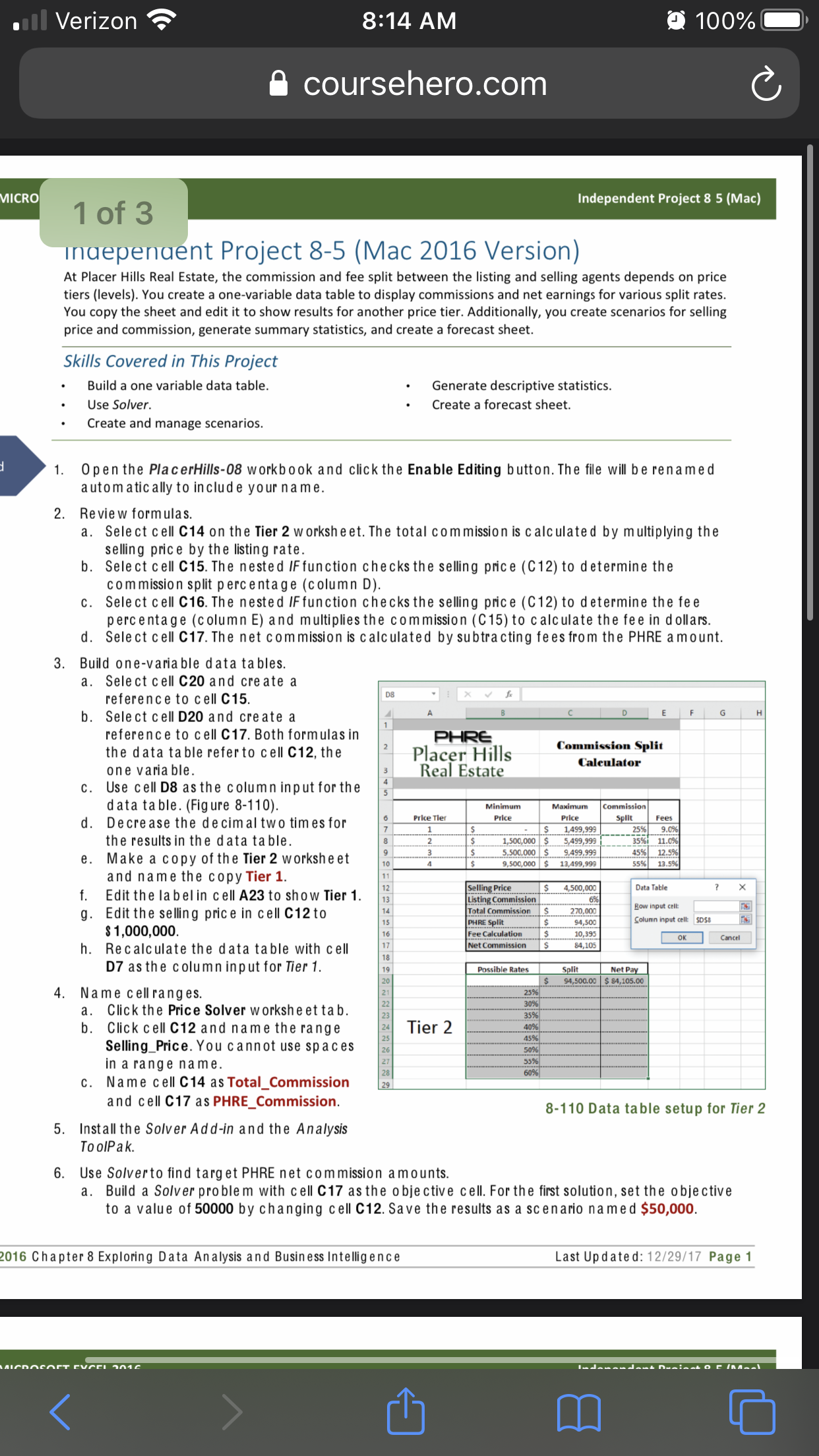
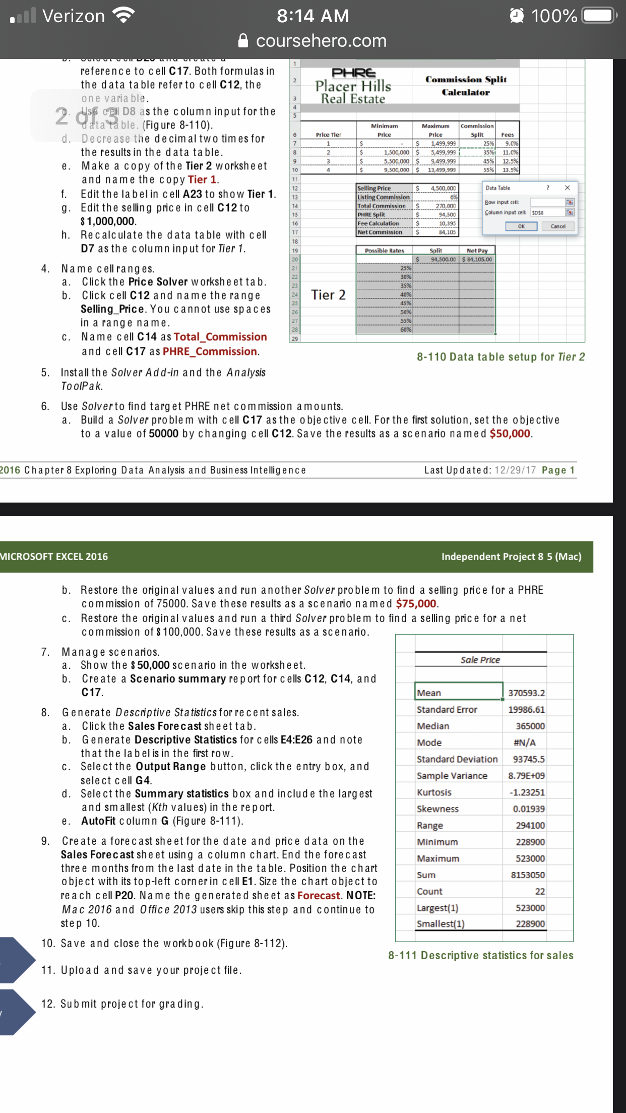
Verizon 8:14 AM 100% coursehero.com MICRO 1 of 3 Independent Project 8 5 (Mac) Independent Project 8-5 (Mac 2016 Version) At Placer Hills Real Estate, the commission and fee split between the listing and selling agents depends on price tiers (levels). You create a one-variable data table to display commissions and net earnings for various split rates. You copy the sheet and edit it to show results for another price tier. Additionally, you create scenarios for selling price and commission, generate summary statistics, and create a forecast sheet. Skills Covered in This Project Build a one variable data table. Generate descriptive statistics. Use Solver. Create a forecast sheet. Create and manage scenarios. 1. Open the PlacerHills-08 workbook and click the Enable Editing button. The file will be renamed automatically to include your name. 2. Review formulas. Select cell C14 on the Tier 2 worksheet. The total commission is calculated by multiplying the selling price by the listing rate. b . Select cell C15. The nested IF function checks the selling price (C12) to determine the commission split percentage (column D). C. Select cell C16. The nested IF function checks the selling price (C12) to determine the fee percentage (column E) and multiplies the commission (C15) to calculate the fee in dollars. d. Select cell C17. The net commission is calculated by subtracting fees from the PHRE amount. 3. Build one-variable data tables. a. Select cell C20 and create a reference to cell C15. I X V & Select cell D20 and create a N -L G reference to cell C17. Both formulas in the data table refer to cell C12, the PHRE Placer Hills Commission Split one variable. Real Estate Calculator C. Use cell D8 as the column input for the data table. (Figure 8-110). Minimum Maximum Commission d. Decrease the decimal two times for Price Tier Price Price Split Fees the results in the data table. 1,499,99 25% 9.0% 1,500,000 $ 5,499,999 35%i 11.0% e. Make a copy of the Tier 2 worksheet 5.500.000 S 9,499,999 45% 12.5% 9,500,000 $ 13,499,999 55% 13.5% and name the copy Tier 1. f. Edit the label in cell A23 to show Tier 1. Selling Price 4,500,000 Data Table X Listing Commission | 6% Edit the selling price in cell C12 to Total Commission 270,000 Row input cell: $ 1,000,000. PHRE Split 94,500 Column input cell: SDS8 Fee Calculation 10,395 h. Recalculate the data table with cell Net Commission 84,105 OK Cancel D7 as the column input for Tier 1. Possible Rates Split Net Pay S 94,500.00 | $ 84,105.00 4. Name cellranges. 2596 a. Click the Price Solver worksheet tab. 30% b. Click cell C12 and name the range Tier 2 35% 40% Selling_Price. You cannot use spaces 45% 50% in a range name. 53% C. Name cell C14 as Total_Commission 60% and cell C17 as PHRE_Commission. 8-110 Data table setup for Tier 2 5. Install the Solver Add-in and the Analysis ToolPak. 6. Use Solverto find target PHRE net commission amounts. a. Build a Solver problem with cell C17 as the objective cell. For the first solution, set the objective to a value of 50000 by changing cell C12. Save the results as a scenario named $50,000. 016 Chapter 8 Exploring Data Analysis and Business Intelligence Last Updated: 12/29/17 Page 1 MICROCAPT FUSEI 2016 mVerizon 8:14 AM 100% a coursehero.com reference to cell C17. Both formulas in the data table refer to cell C12, the N PHRE Placer Hills Commission Split one variable. 2. CSF Cell D8 as the column input for the Real Estate Calculator data table. (Figure 8-110). Minimum Maximum Commission d. Decrease the decimal two times for Price Tier Price price Split Fees the results in the data table. 1,499,999 25% 9.0% 1,500,000 $ 5,499,999 35%1 11.0% e. Make a copy of the Tier 2 worksheet 5.500.000 S 9.499,999 45% 12.5% 9,500,000 $ 13,499,999 55% 13.5% and name the copy Tier 1. f. Edit the label in cell A23 to show Tier 1. Selling Price 4,500,000 Data Table X Listing Commission Edit the selling price in cell C12 to Total Commission 270.000 Row input cell: 94,500 Column input cell: SDSS $ 1,000,000. PHRE Split .S Fee Calculation $ 10,595 h. Recalculate the data table with cell Net Commission 84,105 OK Cancel D7 as the column input for Tier 1. Possible Rates Split Net Pay 94,500.00 $ 84,105.00 4. Name cellranges. 25% a. Click the Price Solver worksheet tab. 30% b. Click cell C12 and name the range Tier 2 35% 40% Selling_Price. You cannot use spaces 45% 509% in a range name. 53% 60% C. Name cell C14 as Total_Commission and cell C17 as PHRE_Commission. 8-110 Data table setup for Tier 2 5. Install the Solver Add-in and the Analysis ToolPak. 6. Use Solverto find target PHRE net commission amounts. a. Build a Solver problem with cell C17 as the objective cell. For the first solution, set the objective to a value of 50000 by changing cell C12. Save the results as a scenario named $50,000. 016 Chapter 8 Exploring Data Analysis and Business Intelligence Last Updated: 12/29/17 Page 1 MICROSOFT EXCEL 2016 Independent Project 8 5 (Mac) b. Restore the original values and run another Solver problem to find a selling price for a PHRE commission of 75000. Save these results as a scenario named $75,000. C. Restore the original values and run a third Solver problem to find a selling price for a net commission of $ 100,000. Save these results as a scenario. 7. Manage scenarios. a. Show the $ 50,000 scenario in the worksheet. Sale Price b. Create a Scenario summary report for cells C12, C14, and C17. Mean 370593.2 8. Generate Descriptive Statistics for recent sales. Standard Error 19986.61 a. Click the Sales Forecast sheet tab. Median 365000 b. Generate Descriptive Statistics for cells E4:E26 and note Mode #N/A that the label is in the first row. C. Select the Output Range button, click the entry box, and Standard Deviation 93745.5 select cell G4. Sample Variance 8.79E+09 d. Select the Summary statistics box and include the largest Kurtosis -1.23251 and smallest (Kth values) in the report. Skewness 0.01939 e. AutoFit column G (Figure 8-111). Range 294100 9. Create a forecast sheet for the date and price data on the Minimum 228900 Sales Forecast sheet using a column chart. End the forecast three months from the last date in the table. Position the chart Maximum 523000 object with its top-left corner in cell E1. Size the chart object to Sum 8153050 reach cell P20. Name the generated sheet as Forecast. NOTE: Count 22 Mac 2016 and Office 2013 users skip this step and continue to Largest(1) 523000 step 10. Smallest(1) 228900 10. Save and close the workbook (Figure 8-112). 8-111 Descriptive statistics for sales 11. Upload and save your project file. 12. Submit project for grading