I need help with 5

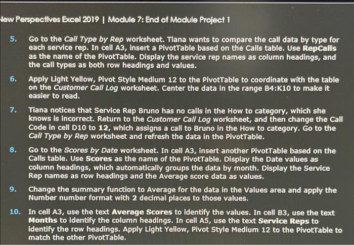
5. Go to the Call Type by Rep worksheet. Tiana wants to compare the call data by type for each service rep. In cell A3, insert a PivotTable based on the Calls table. Use RepCalls as the name of the PivotTable. Display the service rep names as column headings, and the call types as both row headings and values. 6. Apply Light Yellow, Pivot Style Medium 12 to the PivotTable to coordinate with the table on the Customer Call Log worksheet. Center the data in the range B4:K10 to make it easier to read. 7. Tiana notices that Service Rep Bruno has no calls in the How to category, which she knows is incorrect. Return to the Customer Call Log worksheet, and then change the Call Code in cell D10 to 12, which assigns a call to Bruno in the How to category. Go to the Call Type by Rep worksheet and refresh the data in the PivotTable. 8. Go to the Scores by Date worksheet. In cell A3, insert another PivotTable based on the Calls table. Use Scores as the name of the PivotTable. Display the Date values as column headings, which automatically groups the data by month. Display the Service Rep names as row headings and the Average score data as values. 9. Change the summary function to Average for the data in the Values area and apply the Number number format with 2 decimal places to those values. 10. In cell A3, use the text Average Scores to identify the values. In cell B3, use the text Months to identify the column headings. In cell A5, use the text Service Reps to identify the row headings. Apply Light Yellow, Pivot Style Medium 12 to the PivotTable to match the other PivotTable. 5. Go to the Call Type by Rep worksheet. Tiana wants to compare the call data by type for each service rep. In cell A3, insert a PivotTable based on the Calls table. Use RepCalls as the name of the PivotTable. Display the service rep names as column headings, and the call types as both row headings and values. 6. Apply Light Yellow, Pivot Style Medium 12 to the PivotTable to coordinate with the table on the Customer Call Log worksheet. Center the data in the range B4:K10 to make it easier to read. 7. Tiana notices that Service Rep Bruno has no calls in the How to category, which she knows is incorrect. Return to the Customer Call Log worksheet, and then change the Call Code in cell D10 to 12, which assigns a call to Bruno in the How to category. Go to the Call Type by Rep worksheet and refresh the data in the PivotTable. 8. Go to the Scores by Date worksheet. In cell A3, insert another PivotTable based on the Calls table. Use Scores as the name of the PivotTable. Display the Date values as column headings, which automatically groups the data by month. Display the Service Rep names as row headings and the Average score data as values. 9. Change the summary function to Average for the data in the Values area and apply the Number number format with 2 decimal places to those values. 10. In cell A3, use the text Average Scores to identify the values. In cell B3, use the text Months to identify the column headings. In cell A5, use the text Service Reps to identify the row headings. Apply Light Yellow, Pivot Style Medium 12 to the PivotTable to match the other PivotTable