I need help with the ones in red. step by step instructions please.

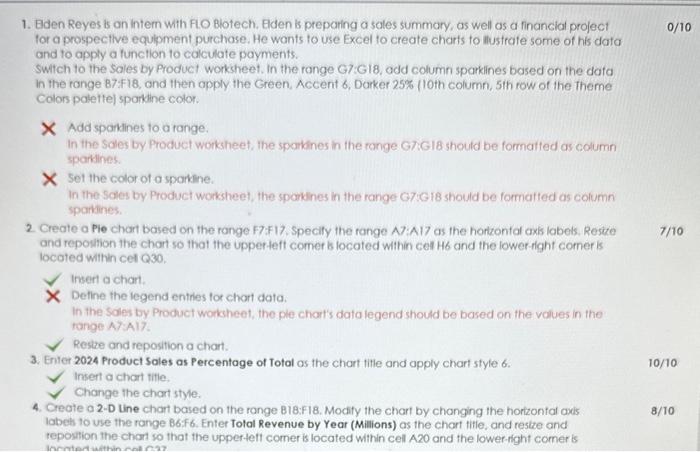
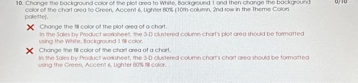
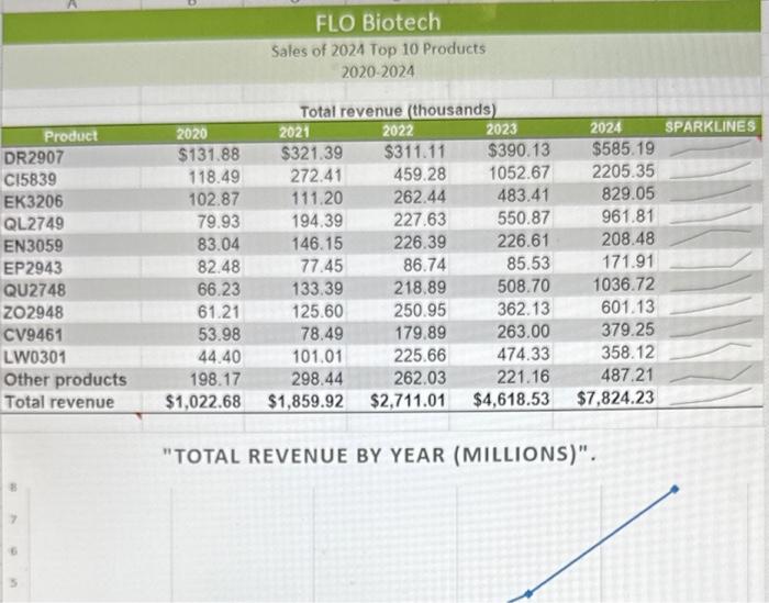
1. Bden Reyes is an intem with FiO Blotech. Elden is preparing a soles summary, as well as a financial project 0/10 tor a prospectlve equipment purchose. He wants to use Excel to create charts to llustrate some of his data and to apply a function to colculate payments. Switch to the Sales by Product worksheet. In the range G7:GI8, odd column sparkines based on the data in the range 87:418, and then apply the Green, Accent 6 , Darker 25% (10th column, 5th row of the theme Colors palettej sparkine color. X Add sparkines to a range. In the Soles by Product worksheet, the sparkines in the ronge G7Gib shoutd be formatted as column sparkines. Set the color of o sparkine. In the Soles by Product worksheet, the sparkines in the range G7:G 18 should be formatied as column sparkines. 2. Create a Pie chart based on the range F7:F17. Specily the range A7:A17 as the horizonfal axis labets. Resize 7/10 and repowhion the chart so that the upperteft comer b locoted within cel Hb and the lower-fight comer is locoted within cet Q30. Insert a chart. Define the legend entries tor chart data. In the Sales by Product workseet, the ple chart's data legend should be based on the volues in the tange A7:A17 Restre and reposition a chart. 3. Eriter 2024 Product Sales as Percentage of Total as the chart title and opply chart style 6. 10/10 Insert a chart title. Change the chart style. 4. Create a 2-D Line chart based on the range B18:F18. Modity the chart by changing the hortzontal adis 8/10 labeb to vse the range B6F6, Enter Tolal Revenue by Year (Millions) as the chart tifle, and restre and repostion the chart so that the upperteft comer is located within cell A20 and the lower-fght comer is 10. Change the background color of the plot area to White, Background I and then change the background color of the chart area to Green, Accent 6 , Lighter 80% (10th column. 2nd row in the Theme Colors palette). X Change the fil color of the plot area of a chart. In the Sales by Product worksheet, the 3-D clustered column chart's plot area should be formatted using the White, Background 1 fil color. * Change the fill color of the chart area of a chart. In the Sales by Product worksheet, the 3.D clustered column chants chort area should be formatted using the Green, Accent 6, Lighter 80% fil color: "TOTAL REVENUE BY YEAR (MILLIONS)". 1. Bden Reyes is an intem with FiO Blotech. Elden is preparing a soles summary, as well as a financial project 0/10 tor a prospectlve equipment purchose. He wants to use Excel to create charts to llustrate some of his data and to apply a function to colculate payments. Switch to the Sales by Product worksheet. In the range G7:GI8, odd column sparkines based on the data in the range 87:418, and then apply the Green, Accent 6 , Darker 25% (10th column, 5th row of the theme Colors palettej sparkine color. X Add sparkines to a range. In the Soles by Product worksheet, the sparkines in the ronge G7Gib shoutd be formatted as column sparkines. Set the color of o sparkine. In the Soles by Product worksheet, the sparkines in the range G7:G 18 should be formatied as column sparkines. 2. Create a Pie chart based on the range F7:F17. Specily the range A7:A17 as the horizonfal axis labets. Resize 7/10 and repowhion the chart so that the upperteft comer b locoted within cel Hb and the lower-fight comer is locoted within cet Q30. Insert a chart. Define the legend entries tor chart data. In the Sales by Product workseet, the ple chart's data legend should be based on the volues in the tange A7:A17 Restre and reposition a chart. 3. Eriter 2024 Product Sales as Percentage of Total as the chart title and opply chart style 6. 10/10 Insert a chart title. Change the chart style. 4. Create a 2-D Line chart based on the range B18:F18. Modity the chart by changing the hortzontal adis 8/10 labeb to vse the range B6F6, Enter Tolal Revenue by Year (Millions) as the chart tifle, and restre and repostion the chart so that the upperteft comer is located within cell A20 and the lower-fght comer is 10. Change the background color of the plot area to White, Background I and then change the background color of the chart area to Green, Accent 6 , Lighter 80% (10th column. 2nd row in the Theme Colors palette). X Change the fil color of the plot area of a chart. In the Sales by Product worksheet, the 3-D clustered column chart's plot area should be formatted using the White, Background 1 fil color. * Change the fill color of the chart area of a chart. In the Sales by Product worksheet, the 3.D clustered column chants chort area should be formatted using the Green, Accent 6, Lighter 80% fil color: "TOTAL REVENUE BY YEAR (MILLIONS)