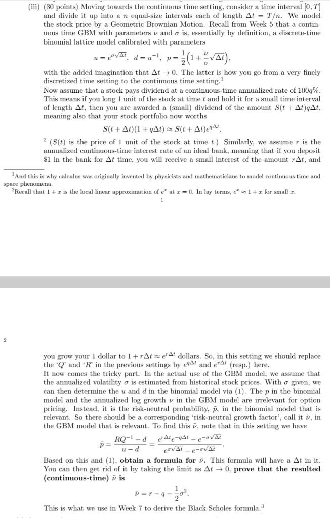
Question: (iii) (30 points) Moving towards the continuous time setting, consider a time interval [0,T] and divide it up into a n equal-size intervals each of

(iii) (30 points) Moving towards the continuous time setting, consider a time interval [0,T] and divide it up into a n equal-size intervals each of length At = T. We model the stock price by a Geometric Brownian Motion. Recall from Week 5 that a contin- uous time GBM with parameters vand o is, essentially by definition, a discrete-time binomial lattice model calibrated with parameters u= VAI deu-1 P= - 1/1 (1 + At), with the added imagination that At +0. The latter is how you go from a very finely discretized time setting to the continuous time setting. Now assume that a stock pays dividend at a continuous-time annualized rate of 100%. This means if you long 1 unit of the stock at time t and hold it for a small time interval of length At, then you are awarded a (small) dividend of the amount S(t + AtqAt, meaning also that your stock portfolio now worths S(t + At)(1+qAt) S(t + Atlet 2 (S(t) is the price of 1 unit of the stock at time t.) Similarly, we assume r is the annualized continuous-time interest rate of an ideal bank, meaning that if you deposit $1 in the bank for At time, you will receive a small interest of the amount rAt, and And this is why calculus was originally invented by physicists and mathematicians to model continuous time and space phenomena Recall that 1+r is the local linear approximation of eat 1 = 0. In lay terms, 1 +r for small r. 1 2 you grow your 1 dollar to 1+rAtert dollars. So, in this setting we should replace the 'Q' and 'R' in the previous settings by e91 and erAt(resp.) here. It now comes the tricky part. In the actual use of the GBM model, we assume that the annualized volatility o is estimated from historical stock prices. With a given, we can then determine the u and d in the binomial model via (1). The p in the binomial model and the annualized log growth v in the GBM model are irrelevant for option pricing. Instead, it is the risk-neutral probability, p, in the binomial model that is relevant. So there should be a corresponding 'risk-neutral growth factor', call it i, in the GBM model that is relevant. To find this i, note that in this setting we have RO-1-d etAle-Af- e-ovar p= / e- Based on this and (1), obtain a formula for . This formula will have a At in it. You can then get rid of it by taking the limit as At 0, prove that the resulted (continuous-time) i is ud =r-9- This is what we use in Week 7 to derive the Black-Scholes formula. (iii) (30 points) Moving towards the continuous time setting, consider a time interval [0,T] and divide it up into a n equal-size intervals each of length At = T. We model the stock price by a Geometric Brownian Motion. Recall from Week 5 that a contin- uous time GBM with parameters vand o is, essentially by definition, a discrete-time binomial lattice model calibrated with parameters u= VAI deu-1 P= - 1/1 (1 + At), with the added imagination that At +0. The latter is how you go from a very finely discretized time setting to the continuous time setting. Now assume that a stock pays dividend at a continuous-time annualized rate of 100%. This means if you long 1 unit of the stock at time t and hold it for a small time interval of length At, then you are awarded a (small) dividend of the amount S(t + AtqAt, meaning also that your stock portfolio now worths S(t + At)(1+qAt) S(t + Atlet 2 (S(t) is the price of 1 unit of the stock at time t.) Similarly, we assume r is the annualized continuous-time interest rate of an ideal bank, meaning that if you deposit $1 in the bank for At time, you will receive a small interest of the amount rAt, and And this is why calculus was originally invented by physicists and mathematicians to model continuous time and space phenomena Recall that 1+r is the local linear approximation of eat 1 = 0. In lay terms, 1 +r for small r. 1 2 you grow your 1 dollar to 1+rAtert dollars. So, in this setting we should replace the 'Q' and 'R' in the previous settings by e91 and erAt(resp.) here. It now comes the tricky part. In the actual use of the GBM model, we assume that the annualized volatility o is estimated from historical stock prices. With a given, we can then determine the u and d in the binomial model via (1). The p in the binomial model and the annualized log growth v in the GBM model are irrelevant for option pricing. Instead, it is the risk-neutral probability, p, in the binomial model that is relevant. So there should be a corresponding 'risk-neutral growth factor', call it i, in the GBM model that is relevant. To find this i, note that in this setting we have RO-1-d etAle-Af- e-ovar p= / e- Based on this and (1), obtain a formula for . This formula will have a At in it. You can then get rid of it by taking the limit as At 0, prove that the resulted (continuous-time) i is ud =r-9- This is what we use in Week 7 to derive the Black-Scholes formula
Step by Step Solution
There are 3 Steps involved in it

Get step-by-step solutions from verified subject matter experts


