Im needing more help with the formulas and which given numbers to use. Any help would be appreciated!!

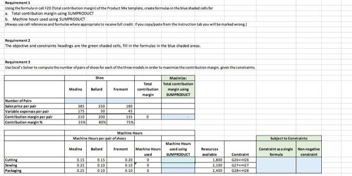
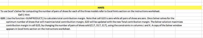
Pequirement 1 Using the formula in cell F20 (Total contribution margin) of the Product Mix template, create formulas in the blue shaded cells for . Total contribution margin using 5UMPRODUCT b. Machine hours used using SUMPRODUCT \{Aways usecell references and formulas where appropriate to receive full credit. If you copy/paste from the instruction tab you will be marked wrong.) Reguirement 2 The objective and constraints headings are the green shaded cells, fill in the formulas in the blue shaded areas. Requirement 3 Use Excel's Solver to compute the number of pairs of shoes for each of the three models in order to maimize the contribution marein, given the constraints. HINTS To use Excel's Solver for computing the number of pairs of shoes for each of the three models refer to Excel hints section on the Instructions worksheet. Cell | Hint: G20 | Use the function =SUMPRODUCT() to calculate total contribution margin. Note that cell G20 is zero while all pairs of shoes are zero. Once Solver solves for the optimum number of shoes that will maximize total contribuition margin, G20 will be updated with the new Total contribution margin. The Solver solution maximizes contribution margin in cell G20, by changing the number of pairs of shoes sold (C17, D17, E17), using the constraints in columns J and K. A copy of the Solver window appears in Excel hints section on the instructions workshees