I'm running into problems with questions following this initial question. I don't know where I'm getting it wrong. And I also don't know how to print the correlation coefficient for the data.

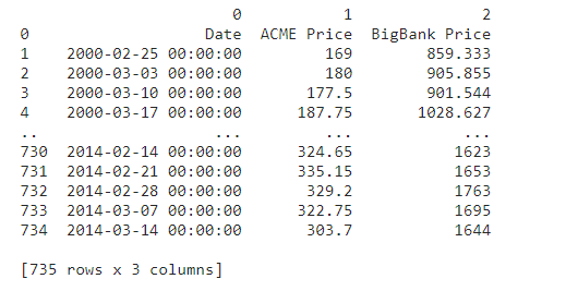This is the csv data file we have.

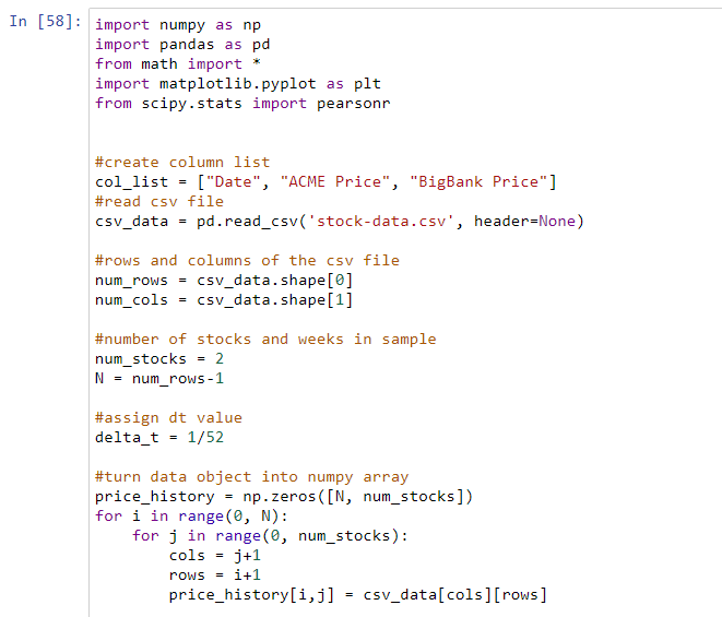
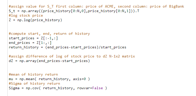
Below are my codes,

Please help me, I can't proceed with the rest of the questions for this exercise ;(((

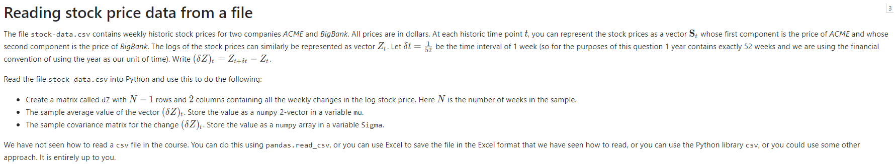
1 2 3 4 0 1 2 Date ACME Price BigBank Price 2000-02-25 00:00:00 169 859.333 2000-03-03 00:00:00 180 905.855 2000-03-10 00:00:00 177.5 901.544 2000-03-17 00:00:00 187.75 1028.627 730 731 732 733 734 2014-02-14 00:00:00 2014-02-21 00:00:00 2014-02-28 00:00:00 2014-03-07 00:00:00 2014-03-14 00:00:00 324.65 335.15 329.2 322.75 303.7 1623 1653 1763 1695 1644 [735 rows x 3 columns ] Reading stock price data from a file The file stock-data.csv contains weekly historic stock prices for two companies ACME and BigBank. All prices are in dollars. At each historic time point t, you can represent the stock prices as a vector St whose first component is the price of ACME and whose second component is the price of BigBank. The logs of the stock prices can similarly be represented as vector Z+. Let dt = 3 be the time interval of 1 week (so for the purposes of this question 1 year contains exactly 52 weeks and we are using the financial convention of using the year as our unit of time). Write (SZ)= Z+ot 27. Read the file stock-data.csv into Python and use this to do the following: Create a matrix called dZ with N 1 rows and 2 columns containing all the weekly changes in the log stock price. Here N is the number of weeks in the sample. The sample average value of the vector (8Z). Store the value as a numpy 2-vector in a variable mu. The sample covariance matrix for the change (8Z). Store the value as a numpy array in a variable Sigma. We have not seen how to read a csv file in the course. You can do this using pandas.read_csv, or you can use Excel to save the file in the Excel format that we have seen how to read, or you can use the Python library csv, or you could use some other approach. It is entirely up to you. In [58]: import numpy as np import pandas as pd from math import import matplotlib.pyplot as plt from scipy.stats import pearson #create column list col_list ["Date", "ACME Price", "BigBank Price"] #read csv file csv_data = pd.read_csv('stock-data.csv', header=None) #rows and columns of the csv file num_rows csv_data.shape[@] num_cols csv_data. shape [1] #number of stocks and weeks in sample num_stocks 2 N = num_rows-1 #assign dt value delta_t = 1/52 #turn data object into numpy array price_history np.zeros([N, num_stocks]) for i in range(0, N): for j in range(0, num_stocks): cols j+1 i+1 price_history[i,j] csv_data[cols][rows] rows #assign value for S T first column: price of ACME, second column: price of BigBank S_t = np.array((price_history[O:N, 0],price_history[0:N,1])).T #log stock price Z np.log(price_history) #compute start, end, return of history start_prices = Z[:-1,:] end_prices = Z[1:,:] return_history = (end_prices-start_prices) /start_prices #assign difference of log of stock price to dz N-1x2 matrix dZ - np.array(end_prices-start_prices) #mean of history return mu = np.mean( return_history, axis=0 ) #Sigma of history return Sigma np.cov( return_history, rowvar=False) 1 2 3 4 0 1 2 Date ACME Price BigBank Price 2000-02-25 00:00:00 169 859.333 2000-03-03 00:00:00 180 905.855 2000-03-10 00:00:00 177.5 901.544 2000-03-17 00:00:00 187.75 1028.627 730 731 732 733 734 2014-02-14 00:00:00 2014-02-21 00:00:00 2014-02-28 00:00:00 2014-03-07 00:00:00 2014-03-14 00:00:00 324.65 335.15 329.2 322.75 303.7 1623 1653 1763 1695 1644 [735 rows x 3 columns ] Reading stock price data from a file The file stock-data.csv contains weekly historic stock prices for two companies ACME and BigBank. All prices are in dollars. At each historic time point t, you can represent the stock prices as a vector St whose first component is the price of ACME and whose second component is the price of BigBank. The logs of the stock prices can similarly be represented as vector Z+. Let dt = 3 be the time interval of 1 week (so for the purposes of this question 1 year contains exactly 52 weeks and we are using the financial convention of using the year as our unit of time). Write (SZ)= Z+ot 27. Read the file stock-data.csv into Python and use this to do the following: Create a matrix called dZ with N 1 rows and 2 columns containing all the weekly changes in the log stock price. Here N is the number of weeks in the sample. The sample average value of the vector (8Z). Store the value as a numpy 2-vector in a variable mu. The sample covariance matrix for the change (8Z). Store the value as a numpy array in a variable Sigma. We have not seen how to read a csv file in the course. You can do this using pandas.read_csv, or you can use Excel to save the file in the Excel format that we have seen how to read, or you can use the Python library csv, or you could use some other approach. It is entirely up to you. In [58]: import numpy as np import pandas as pd from math import import matplotlib.pyplot as plt from scipy.stats import pearson #create column list col_list ["Date", "ACME Price", "BigBank Price"] #read csv file csv_data = pd.read_csv('stock-data.csv', header=None) #rows and columns of the csv file num_rows csv_data.shape[@] num_cols csv_data. shape [1] #number of stocks and weeks in sample num_stocks 2 N = num_rows-1 #assign dt value delta_t = 1/52 #turn data object into numpy array price_history np.zeros([N, num_stocks]) for i in range(0, N): for j in range(0, num_stocks): cols j+1 i+1 price_history[i,j] csv_data[cols][rows] rows #assign value for S T first column: price of ACME, second column: price of BigBank S_t = np.array((price_history[O:N, 0],price_history[0:N,1])).T #log stock price Z np.log(price_history) #compute start, end, return of history start_prices = Z[:-1,:] end_prices = Z[1:,:] return_history = (end_prices-start_prices) /start_prices #assign difference of log of stock price to dz N-1x2 matrix dZ - np.array(end_prices-start_prices) #mean of history return mu = np.mean( return_history, axis=0 ) #Sigma of history return Sigma np.cov( return_history, rowvar=False)