Im stuck on #4,7,10 and cant really do the other problems without solving those. Thank you for any help

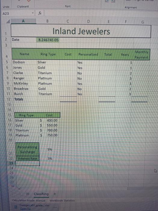
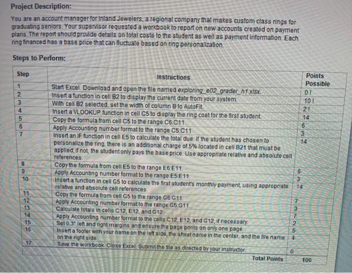
31 TE Undo Cipboard Font Alignment A23 A F G Inland Jewelers Date Nm 8.24674E-05 Name Ring Type Cost Personalized Total Years Monthly Payment Yes 1 1 Silver Gold Titanium Platinum Platinum Gold Titanium Yes No No Yes No Yes mm N 3 5 Dodson 6 Jones Clarke 8 Ranger 9 McKinley 10 Broadnax 11 Burch 12 Totals 13 14 15 Bing Type 16 Silver 17 Gold 18 Titanium 19 Platinum 20 $ S S $ Cost 400.00 550.00 700.00 750.00 Personalizing Surcharge 5% Interest Rate 396 21 22 23 24 25 26 27 Class Ring Workbook Statistics Calculation Moder Manual Castigan 01.grade Project Description: You are an account manager for Inland Jewelers, a regional company that makes custom class rings for graduating seniors. Your supervisor requested a workbook to report on new accounts created on payment plans. The report should provide details on total costs to the student as well as payment information. Each ring financed has a base price that can fluctuate based on ring personalization Steps to Perform: Step 102 1 2 3 4 5 6 7 8 9 Points Instructions Possible Start Excel. Download and open the file named exploring_e02_gradec_n1 xlsx 01 Insert a function in cell 82 to display the current date from your system With cell B2 selected, set the width of column B to AutoFit 21 Insert a VLOOKUP function in cell C5 to display the ring cost for the first student 14 Copy the formula from cell C5 to the range C6:011. 6 Apply Accounting number format to the range C5C11 3 Insert an IF function in cell E5 to calculate the total due. If the student has chosen to 14 personalize the ring, there is an additional charge of 5% located in cell B21 that must be applied: If not, the student only pays the base price. Use appropriate relative and absolute cell references Copy the formula from cell E5 to the range E6E11 Apply Accounting number format to the range E5E11 Insert a function in cell G5 to calculate the first student's monthly payment using appropriate relative and absolute cell references. Copy the formula from cell G5 to the range 66:611. Apply Accounting number format to the range G5 G11 3 Calculate totals in cells C12, E12, and G12. Apply Accounting number format to the cells C12, E12, and G12, if necessary: Set 0.3" In and right margins and ensure the page prints on only one page 5 Insert a footer with your name on the left side, the sheet name in the center, and the file name on the right side Save the workbook Close Excel. Submit the file as directed by your instructor 0 Total Points 100 10 6 3 14 7 11 12 13 14 15 16 7 2 4 17