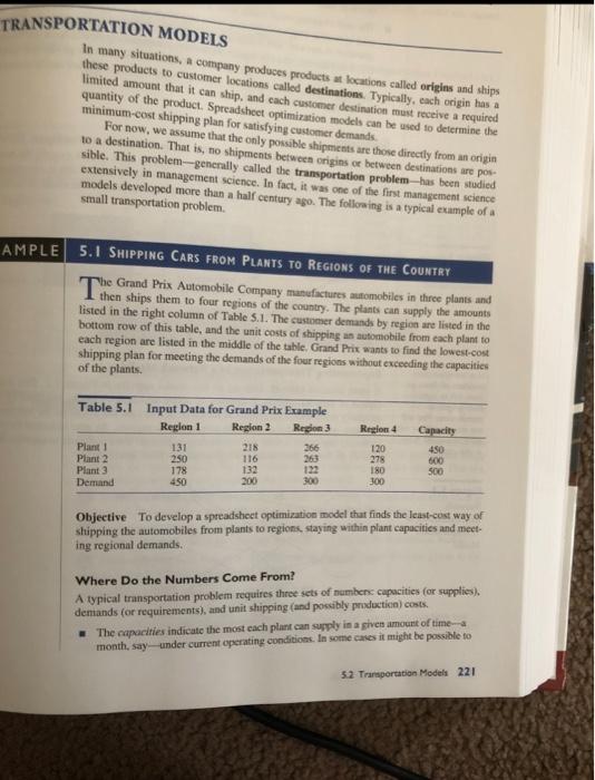
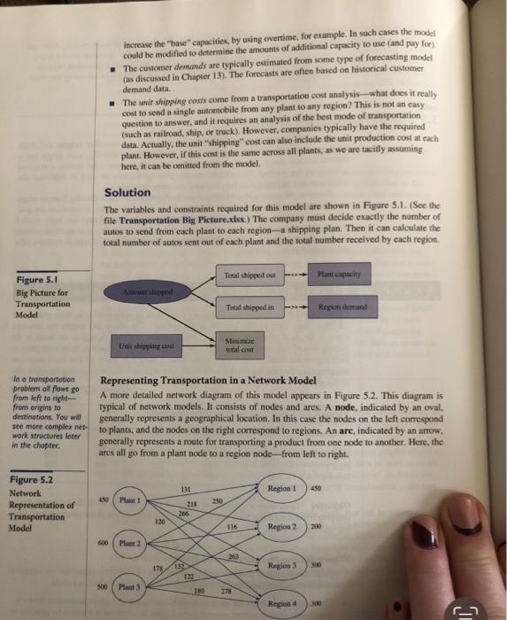
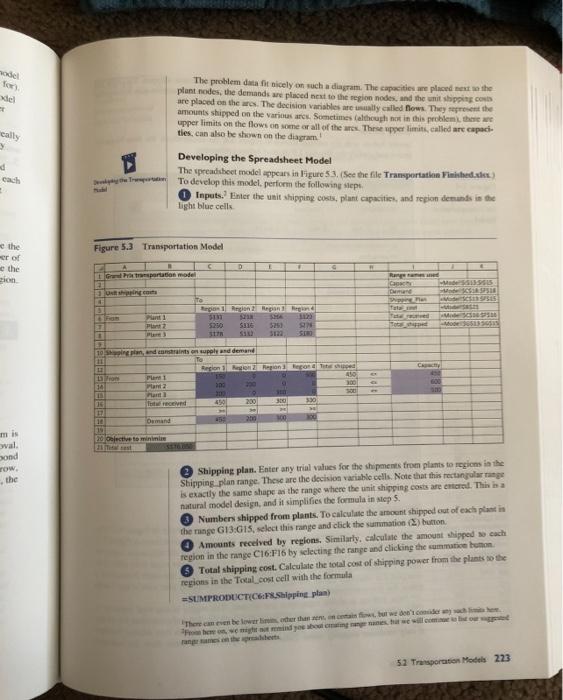
In a transportation problem such as Example 5.1, if a route is not being used in the optimal solution, then the reduced cost is negative and indicates how much less the unit shipping cost would have to be before the route can be used. o the reduced cost is O the reduced cost is positive and indicates how much less the unit shipping cost would have to be before the route can be used. O the reduced cost is 1E30 TRANSPORTATION MODELS In many situations, a company produces products at locations called origins and ships these products to customer locations called destinations. Typically, each origin has a limited amount that it can ship, and cach customer destination must receive a required quantity of the product. Spreadsheet optimization models can be used to determine the minimum-cost shipping plan for satisfying customer demands For now, we assume that the only possible shipments are those directly from an origin to a destination. That is, no shipments between origins or between destinations are pos sible. This problem-generally called the transportation problem has been studied extensively in management Science. In fact, it was one of the first management science models developed more than a half century ago. The following is a typical example of a small transportation problem. AMPLE 5.1 SHIPPING CARS FROM PLANTS TO REGIONS OF THE COUNTRY T. The Grand Prix Automobile Company manufactures automobiles in three plants and then ships them to four regions of the country. The plants can supply the amounts listed in the right column of Table 5.1. The customer demands by region are listed in the bottom row of this table, and the unit costs of shipping an automobile from each plant to each region are listed in the middle of the table. Grand Prix wants to find the lowest-cost shipping plan for meeting the demands of the four regions without exceeding the capacities of the plants. Table 5.1 Region 4 Input Data for Grand Prix Example Region 1 Region 2 Region 3 131 218 366 250 116 263 178 132 122 450 200 300 Plant 1 Plant 2 Plant 3 Demand 120 Capacity 450 600 500 278 180 300 Objective To develop a spreadsheet optimization model that finds the least-cost way of shipping the automobiles from plants to regions, staying within plant capacities and meet- ing regional demands. Where Do the Numbers Come From? A typical transportation problem requires three sets of numbers capacities for supplies). demands (or requirements), and unit shipping (and possibly production) costs. The capacities indicate the most cach plant can supply in a given amount of time month, say under current operating conditions. In some cases it might be possible to 52 Transportation Models 221 increase the "hase" capacities, by using overtime, for example. In such cases the model could be modified to determine the amounts of additional capacity to use (and pay for The customer demands are typically estimated from some type of forecasting model (as discussed in Chapter 13). The forecasts are often based on historical customer demand data . The unit shipping costs come from a transportation cost analysis, what does it really cost to send a single automobile from any plant to any region? This is not an easy question to answer, and it requires an analysis of the best mode of transportation (such as railroad, ship, or track). However, companies typically have the required data. Actually, the unit "shipping cost can also include the unit production cost at each plant. However, if this cost is the same across all plants, as we are tacitly assuming here, it can be omitted from the model. Solution The variables and constraints required for this model are shown in Figure 5.1. (See the file Transportation Big Picture.xlsx.) The company must decide exactly the number of autos to send from each plant to cach region- shipping plan. Then it can calculate the total number of nutos sent out of each plant and the total number received by each region. Total shipped out ant capacity Figure 5.1 Big Picture for Transportation Model Amenipped Total shipped in Ropion demand Mineze t shipping cont In a transportation problem all flows from left to right- from origins to destinations. You will see more complex net- work structures loter in the chapter. Representing Transportation in a Network Model A more detailed network diagram of this model appears in Figure 5.2. This diagram is typical of network models. It consists of nodes and ares. A node, indicated by an oval, generally represents a geographical location. In this case the nodes on the left correspond to plants, and the nodes on the right correspond to regions. An arc, indicated by an arrow, generally represents a route for transporting a product from one node to another. Here, the arcs all go from a plant node to a region node--from left to right. 131 Region 1 Figure 5.2 Network Representation of Transportation Model Plant 1 250 218 266 120 116 Region 2 2010 600 X 178 132 Region 3 300 500 Plant 180 VE Region 4 10 1 del for de The problem data fit nicely on such a diagram. The capacities we placed exto the plant modes, the demands are placed next to the region nodes, and the unit shipping.com are placed on the wes. The decision variables are ually called flows. They represent the amounts shipped on the various arcs. Sometimes although not in this problem, there we upper limits on the flows on some or all of the arts. These wpper limits, called are capaci. ties, can also be shown on the diagram! cally ad cach Developing the Spreadsheet Model The spreadsheet model appears in Figure 53. (See the file Transportation mished.de T To develop this model, perform the following steps Inputs. Enter the unit shipping costs, plant capacities, and region demands in the light blue cells Figure 5.3 Transportation Model e the er of the ion GrProportation model Rp VIS SUSISI SIS To Segon ciontapang Plant 1 Part 2 WE MOS SH 5253 AN 1000 10 in and son supply and demand 11 Regionen Reported Plant 650 14 Platz an an 15 Test received 200 330 11 10 Omand 45 20 100 19 20 elective to minimi ond row, the Shipping plan. Enter any trial values for the shipments from plants to regions in the Shipping plan range. These are the decision variable cells. Note that this rectangular range is exactly the same shape as the range where the unit shipping costs are entered. This is a natural model design, and it simplifies the formula in step 5. Numbers shipped from plants. To calculate the amount shipped out of each plant is the range G13:15, select this range and click the summimation (2) button. Amounts received by regions. Similarly, calculate the amount shipped cach region in the range C16:F16 by selecting the range and clicking the summation human Total shipping cost. Calculate the total cost of shipping power from the plants to the regions in the Tocal cost cell with the formula =SUMPRODUCTCPS Shipping plan) There can be lower than info but we'de mig ut midye bones will come to 52 Transportation Models 223 The optimal solution to the original Grand Prix problem (Example 5.1) indicates that with a unit shipping cost of $132, the route from plant 3 to region 2 is evidently too expensive-no autos are shipped along this route. Based on a one-way SolverTable that varies this unit shipping cost from $0 to $130 in increments of $10, what is the highest unit shipping cost that some autos would be shipped along this route. O 10 40 50 O 90 60 O 110 O 20