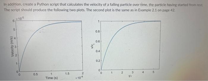
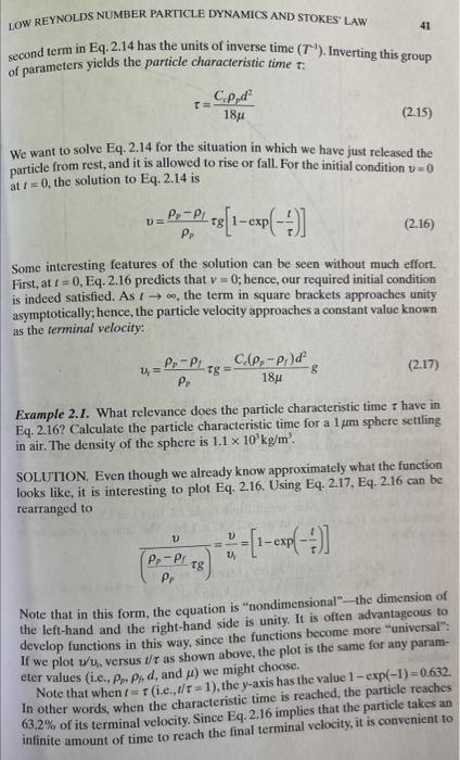
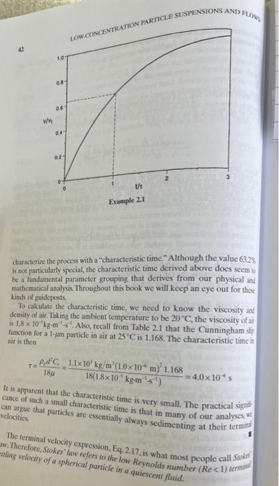
In addition, create a Python script that calculates the velocity of a falling particle over time, the particle having started from rest. The script should produce the following two plots. The second plot is the same as in Example 2.1 on page 42. 610-5 5 Velocity (m/s) NA 0.8 0.6 0.4 0.2 0 0 0.5 1.5 2 0 1 2 3 Time (s) x104 UT LOW REYNOLDS NUMBER PARTICLE DYNAMICS AND STOKES LAW 41 second term in Eq. 2.14 has the units of inverse time (T). Inverting this group of parameters yields the particle characteristic time t: C.pd T = 18 (2.15) We want to solve Eq. 2.14 for the situation in which we have just released the particle from rest, and it is allowed to rise or fall. For the initial condition - 0 at = 0, the solution to Eq. 2.14 is v=P-Prg [1-exp(-)] D= Pp (2.16) Some interesting features of the solution can be seen without much effort. First, at t=0, Eq. 2.16 predicts that v = 0; hence, our required initial condition is indeed satisfied. As too, the term in square brackets approaches unity asymptotically; hence, the particle velocity approaches a constant value known as the terminal velocity: =P-P Pr Tg= CP - P})d g 18 (2.17) Example 2.1. What relevance does the particle characteristic time r have in Eq. 2.16? Calculate the particle characteristic time for a 1 m sphere settling in air. The density of the sphere is 1.1 x 10'kg/m. SOLUTION. Even though we already know approximately what the function looks like, it is interesting to plot Eq. 2.16. Using Eq. 2.17, Eq. 2.16 can be rearranged to 1) Pp-Ps Pr tg Note that in this form, the equation is "nondimensional"--the dimension of the left-hand and the right-hand side is unity. It is often advantageous to develop functions in this way, since the functions become more "universal": If we plot u'u, versus I/T as shown above, the plot is the same for any param- eter values (i.e., P. P. d, and ) we might choose. Note that when = (ie.,t/t=1), the y-axis has the value 1-exp(-1)=0.632. In other words, when the characteristic time is reached, the particle reaches 63.2% of its terminal velocity. Since Eq. 2.16 implies that the particle takes an infinite amount of time to reach the final terminal velocity, it is convenient to 04 02- 1.0 LOW CONCENTRATION PARTICLE SUSPENSIONS AND FLOW 0.8 1/1 Example 2.1 characterize the process with a "characteristic time." Although the value 63.2% is not particularly special, the characteristic time derived above does seem to be a fundamental parameter grouping that derives from our physical and mathematical analysis. Throughout this book we will keep an eye out for these kinds of guideposts To calculate the characteristic time, we need to know the viscosity and density of air. Taking the ambient temperature to be 20C, the viscosity of ar is 1.8 x 10 kg-m. Also, recall from Table 2.1 that the Cunningham sp function for a 1-um particle in air at 25C is 1.168. The characteristic time in air is then T= Pd C 1.1x10' kg/m (1.0x10 m) 1.168 18(1.8x10 kg-ms') 18 =4.0x10 s WC It is apparent that the characteristic time is very small. The practical sign cance of such a small characteristic time is that in many of our analyses, V can argue that particles are essentially always sedimenting at their terminal velocities. w. Therefore, Stokes' law refers to the low Reynolds number (Re