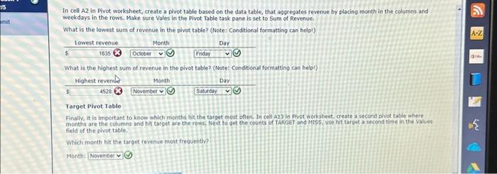
In cell A2 in Pivot worksheet, create a pivot table based on the data table, that aggregates revenue by placing month in the columns and weekdays in the rows. Make sure Vales in the Pivot Table task pane is set to Sum of Revenue. What is the lowest sum of revenue in the pivot table? (Note: Conditional formatting can helpl) What is the highest sum of revenue in the pivot table? (Note: Conditional formatting can helol) Target Pivot Table Finally, it is important to know which months hit the target mest often. In cell A13 in pivot workhest, create a second pivot table where. monthis are the columns and hit target are the rows. Noxt to get the counts of TAKCET and Miss, use hit target a second time in the values field of the pivot table. Which month hit the target revenue most frequentw? Menth: In cell A2 in Pivot worksheet, create a pivot table based on the data table, that aggregates revenue by placing month in the columns and weekdays in the rows. Make sure Vales in the Pivot Table task pane is set to Sum of Revenue. What is the lowest sum of revenue in the pivot table? (Note: Conditional formatting can helpl) What is the highest sum of revenue in the pivot table? (Note: Conditional formatting can helol) Target Pivot Table Finally, it is important to know which months hit the target mest often. In cell A13 in pivot workhest, create a second pivot table where. monthis are the columns and hit target are the rows. Noxt to get the counts of TAKCET and Miss, use hit target a second time in the values field of the pivot table. Which month hit the target revenue most frequentw? Menth