

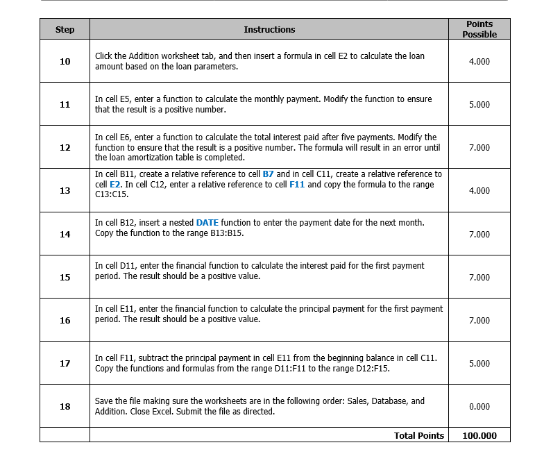
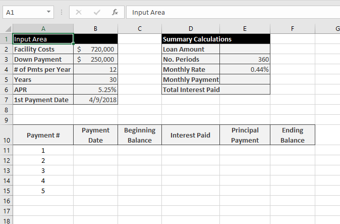
Question: In cell E6, enter a function to calculate the total interest paid after five payments. Modify the function to ensure that the result is a
In cell E6, enter a function to calculate the total interest paid after five payments. Modify the function to ensure that the result is a positive number. The formula will result in an error until the loan amortization table is completed. In cell B11, create a relative reference to cell B7 and in cell C11, create a relative reference to cell E2. In cell C12, enter a relative reference to cell F11 and copy the formula to the range C13:C15.
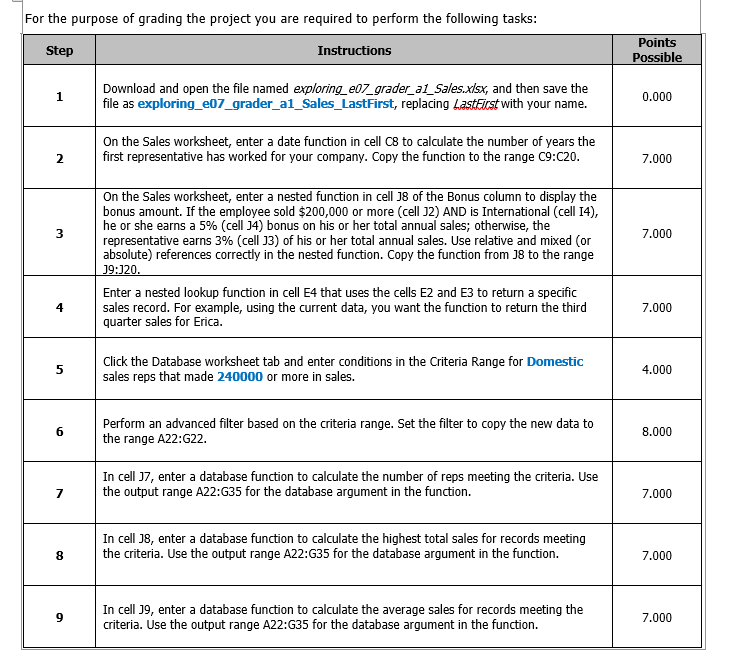
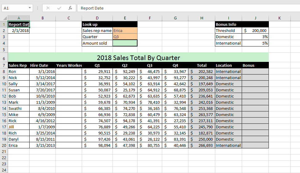
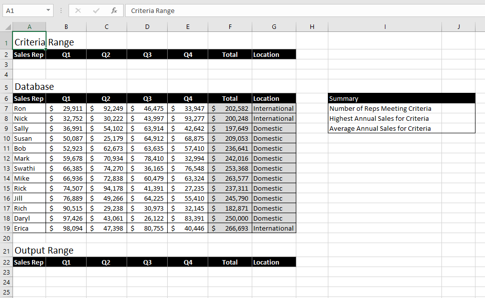
For the purpose of grading the project you are required to perform the following tasks: Points Possible Step Download and open the file named exploring e07 grader a1Sales.xisx, and then save the file as exploring_e07_grader_al_Sales_LastFirst, replacing LastEicst with your name. 0.000 On the Sales worksheet, enter a date function in cell C8 to calculate the number of years the first representative has worked for your company 2 . Copy the function to the range C9:C20 7.000 On the Sales worksheet, enter a nested function in cell 18 of the Bonus column to display the bonus amount. If the employee sold $200,000 or more (cell 12) AND is International (cell 14) he or she earns a 5% (cell 34) bonus on his or her total annual sales; otherwise, the representative earns 3% (cell J3) of his or her total annual sales. Use relative and mixed (or absolute) references correctly in the nested function. Copy the function from J8 to the range 3 7.000 Enter a nested lookup function in cell E4 that uses the cells E2 and E3 to return a specific sales record. For example, using the current data, you want the function to return the third quarter sales for Erica 4 7.000 Click the Database worksheet tab and enter conditions in the Criteria Range for Domestic sales reps that made 240000 or more in sales. 5 4.000 Perform an advanced filter based on the criteria range. Set the filter to copy the new data to the range A22:G22. 6 8.000 In cell 17, enter a database function to calculate the number of reps meeting the criteria. Use the output range A22:G35 for the database argument in the function. 7.000 In cell J8, enter a database function to calculate the highest total sales for records meeting the criteria. Use the output range A22:G35 for the database argument in the function. 8 7.000 In cell 19, enter a database function to calculate the average sales for records meeting the criteria. Use the output range A22:G35 for the database argument in the function. 9 7.000 For the purpose of grading the project you are required to perform the following tasks: Points Possible Step Download and open the file named exploring e07 grader a1Sales.xisx, and then save the file as exploring_e07_grader_al_Sales_LastFirst, replacing LastEicst with your name. 0.000 On the Sales worksheet, enter a date function in cell C8 to calculate the number of years the first representative has worked for your company 2 . Copy the function to the range C9:C20 7.000 On the Sales worksheet, enter a nested function in cell 18 of the Bonus column to display the bonus amount. If the employee sold $200,000 or more (cell 12) AND is International (cell 14) he or she earns a 5% (cell 34) bonus on his or her total annual sales; otherwise, the representative earns 3% (cell J3) of his or her total annual sales. Use relative and mixed (or absolute) references correctly in the nested function. Copy the function from J8 to the range 3 7.000 Enter a nested lookup function in cell E4 that uses the cells E2 and E3 to return a specific sales record. For example, using the current data, you want the function to return the third quarter sales for Erica 4 7.000 Click the Database worksheet tab and enter conditions in the Criteria Range for Domestic sales reps that made 240000 or more in sales. 5 4.000 Perform an advanced filter based on the criteria range. Set the filter to copy the new data to the range A22:G22. 6 8.000 In cell 17, enter a database function to calculate the number of reps meeting the criteria. Use the output range A22:G35 for the database argument in the function. 7.000 In cell J8, enter a database function to calculate the highest total sales for records meeting the criteria. Use the output range A22:G35 for the database argument in the function. 8 7.000 In cell 19, enter a database function to calculate the average sales for records meeting the criteria. Use the output range A22:G35 for the database argument in the function. 9 7.000
Step by Step Solution
There are 3 Steps involved in it

Get step-by-step solutions from verified subject matter experts