In this assignment , you will examine what happens when different sample sizes are used to once ? What if you rolled the die 10 times or 100 times ? You will be given a data file that contains the results from rolling a die 300 times Your task will be to estimate the average n = 1 n = 300 value when a die is rolled using different sample sizes that range from n =1 to n 300

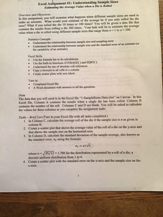
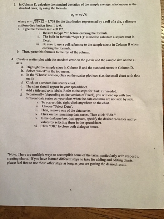
Excel Assignment #1: Understanding Sample Sizes Estimating the Average Value when a Die is Rolled Overview and Objectives In this assignment, you will examine what happens when different sample sizes are used to make an estimate. What would your estimate of the average be if you only rolled the die once? What if you rolled the die 10 times or 100 times? You will be given a data file that contains the results from rolling a die 300 times. Your task will be to estimate the average value when a die is rolled using different sample sizes that range from 1 to 300. Statistics Concepts Understand the relationship between sample size and sampling error Understand the relationship between sample size and the standard error of an estimate (or the variability of an estimate) Excel Skills Use the formula bar to do calculations. Use the built-in functions AVERAGE) and SORTO). Understand the use of absolute cell references Copy a formula to all cells in a column Create scatter plots with axis labels Turn in: Completed Excel file. A Word document with answers to all the questions Data The data that you will need is in the Excel file "I-SampleSizes-Data.xlsx" on Canvas. In this Excel file, Column A contains the results when a single die has been rolled. Column B contains the number of the roll. Columns C and D are blank. You will be asked to calculate the values for these columns as you complete the assignment tasks. Tasks - Brief List (Turn in your Excel file with all tasks completed.) 1. In Column C, calculate the average roll of the die if the sample size is n as given in column B. 2. Create a scatter plot that shows the average value of the roll of a die on the y-axis and that shows the sample size on the horizontal axis. 3. In Column D, calculate the standard deviation of the sample average, also known as the standard error, o, using the formula: 0 g where - /35/12 = 1.708 for the distribution represented by a roll of a die, a discrete uniform distribution from 1 to 6. 4. Create a scatter plot with the standard error on the y-axis and the sample size on the X-axis. Questions (Turn in a Word document with your answers to all questions.) 1. Based on the results of rolling a die 300 times, what do you believe the average value is for the roll of a die? Explain your reasoning. 2. Define the following terms: a. Sampling distribution b. Sampling error c. Standard error 3. Assume a sample average is used as the point estimate for a population mean. Is it guaranteed that as the sample size increases, the sampling error always decreases for every successively larger sample? Why or why not? 4. What happens to the standard error as the sample size increases? Does this make sense? Why or why not? Tasks - Detailed instructions (Use these if you get stuck.) 1. In Column C, calculate the average roll of the die if the sample size is as given in column B. To do this, use the built-in function AVERAGE) to calculate the average. a. Click on the cell in which you would like to do a calculation b. Then, type and enter the formula c. For the first cell (C2), for sample size n-1, you can either A cell reference to the first roll. ii. Directly enter the value from the first roll. iii. The "average of the first cell (i..-AVERAGE(A2)") d. For the second cell (C3), you would like the average of the first two rolls. Use the formula"-AVERAGE(A2:A3)" e. Formulas in Excel can be pasted to an entire column, making your life easier. In this case, however, we want each successive average to include one more cell than the last average so that the sample size increases from 1 to 2 to 3. and so forth. To do this using the AVERAGE formula, we need to keep the first cell reference the same and increment down the last cell reference. We will need to use an absolute reference for the first cell to hold it in place. i. To get an absolute reference, add a "S" in front of both the column (letter) and row (number) of the cell reference. i Hint: A shortcut to adding the absolute reference is to place your curser on that cell reference in the formula bar and hit F4. iii. Your formula for cell C3 should be: "AVERAGE(SAS2:A3)" 1. Once there is an absolute reference on the first cell, you can quickly paste the formula to the entire column by placing the mouse over the lower right-hand corner of the cell containing the formula. A black cross should appear. Double- click on the black cross 2. Create a scatter plot that shows the average value of the roll of a die on the y-axis and that shows the sample size on the horizontal axis. a. Highlight the data in columns B and C that will be included in the chart. (Hint: If you highlight the first few cells of both columns, and then type "Ctrl+Shift+Arrow Down", the entire columns will be highlighted without clicking and dragging. You need to hold down the three keys together, not one at a time, for this shortcut to work.) b. Select "Insert" in the top menu. c. In the "Charts" section, click on the scatter plot icon (ie the small chart with dots on it). d. Click on a smooth line scatter chart. e. The chart should appear in your spreadsheet. Refer to the screenshot in Figure 1 on the next page. f. Add a title for the chart by clicking on the default title and changing it something meaningful. e Add axis labels. Click on the chart. "Add Chart Element should appear at the top of the spreadsheet. When you click on this, you should get the option to add "Axis Titles > Primary Horizontal" and "Axis Titles > Primary Vertical." Refer to the screenshot in Figure 2. 3. In Column D, calculate the standard deviation of the sample average, also known as the standard error, 0using the formula: o = a/VR where = 35/12 1.708 for the distribution represented by a roll of a die, a discrete uniform distribution from 1 to 6. a. Type the formula into cell D2. i. Be sure to type " before entering the formula. ii. The built-in formula "SORTO" is used to calculate a square root in Excel. iii. Be sure to use a cell reference to the sample sizen in Column B when entering the formula. b. Then, paste this formula to the rest of the column. 4. Create a scatter plot with the standard error on the y-axis and the sample size on the x- axis. a. Highlight the sample sizes in Column B and the standard errors in Column D. b. Select "Insert" in the top menu. c. In the "Charts" section, click on the scatter plot icon (.e. the small chart with dots on it). d. Click on a smooth line scatter chart. c. The chart should appear in your spreadsheet. f. Add a title and axis labels. Refer to the steps for Task 2 if needed. g. Occasionally (depending on the version of Excel), you will end up with two different data series on your chart when the data columns are not side by side. i. To correct this, right-click anywhere on the chart. ii. Choose "Select Data". iii. Then, remove one of the data series. iv. Click on the remaining data series. Then click "Edit." V. In the dialogue box that appears, specify the desired x-values and y- values by selecting them in the spreadsheet. vi. Click "OK" to close both dialogue boxes. Note: There are multiple ways to accomplish some of the tasks, particularly with respect to creating charts. If you have learned different steps to take for adding and editing charts, please feel free to use those other steps as long as you are getting the desired result. Excel Assignment #1: Understanding Sample Sizes Estimating the Average Value when a Die is Rolled Overview and Objectives In this assignment, you will examine what happens when different sample sizes are used to make an estimate. What would your estimate of the average be if you only rolled the die once? What if you rolled the die 10 times or 100 times? You will be given a data file that contains the results from rolling a die 300 times. Your task will be to estimate the average value when a die is rolled using different sample sizes that range from 1 to 300. Statistics Concepts Understand the relationship between sample size and sampling error Understand the relationship between sample size and the standard error of an estimate (or the variability of an estimate) Excel Skills Use the formula bar to do calculations. Use the built-in functions AVERAGE) and SORTO). Understand the use of absolute cell references Copy a formula to all cells in a column Create scatter plots with axis labels Turn in: Completed Excel file. A Word document with answers to all the questions Data The data that you will need is in the Excel file "I-SampleSizes-Data.xlsx" on Canvas. In this Excel file, Column A contains the results when a single die has been rolled. Column B contains the number of the roll. Columns C and D are blank. You will be asked to calculate the values for these columns as you complete the assignment tasks. Tasks - Brief List (Turn in your Excel file with all tasks completed.) 1. In Column C, calculate the average roll of the die if the sample size is n as given in column B. 2. Create a scatter plot that shows the average value of the roll of a die on the y-axis and that shows the sample size on the horizontal axis. 3. In Column D, calculate the standard deviation of the sample average, also known as the standard error, o, using the formula: 0 g where - /35/12 = 1.708 for the distribution represented by a roll of a die, a discrete uniform distribution from 1 to 6. 4. Create a scatter plot with the standard error on the y-axis and the sample size on the X-axis. Questions (Turn in a Word document with your answers to all questions.) 1. Based on the results of rolling a die 300 times, what do you believe the average value is for the roll of a die? Explain your reasoning. 2. Define the following terms: a. Sampling distribution b. Sampling error c. Standard error 3. Assume a sample average is used as the point estimate for a population mean. Is it guaranteed that as the sample size increases, the sampling error always decreases for every successively larger sample? Why or why not? 4. What happens to the standard error as the sample size increases? Does this make sense? Why or why not? Tasks - Detailed instructions (Use these if you get stuck.) 1. In Column C, calculate the average roll of the die if the sample size is as given in column B. To do this, use the built-in function AVERAGE) to calculate the average. a. Click on the cell in which you would like to do a calculation b. Then, type and enter the formula c. For the first cell (C2), for sample size n-1, you can either A cell reference to the first roll. ii. Directly enter the value from the first roll. iii. The "average of the first cell (i..-AVERAGE(A2)") d. For the second cell (C3), you would like the average of the first two rolls. Use the formula"-AVERAGE(A2:A3)" e. Formulas in Excel can be pasted to an entire column, making your life easier. In this case, however, we want each successive average to include one more cell than the last average so that the sample size increases from 1 to 2 to 3. and so forth. To do this using the AVERAGE formula, we need to keep the first cell reference the same and increment down the last cell reference. We will need to use an absolute reference for the first cell to hold it in place. i. To get an absolute reference, add a "S" in front of both the column (letter) and row (number) of the cell reference. i Hint: A shortcut to adding the absolute reference is to place your curser on that cell reference in the formula bar and hit F4. iii. Your formula for cell C3 should be: "AVERAGE(SAS2:A3)" 1. Once there is an absolute reference on the first cell, you can quickly paste the formula to the entire column by placing the mouse over the lower right-hand corner of the cell containing the formula. A black cross should appear. Double- click on the black cross 2. Create a scatter plot that shows the average value of the roll of a die on the y-axis and that shows the sample size on the horizontal axis. a. Highlight the data in columns B and C that will be included in the chart. (Hint: If you highlight the first few cells of both columns, and then type "Ctrl+Shift+Arrow Down", the entire columns will be highlighted without clicking and dragging. You need to hold down the three keys together, not one at a time, for this shortcut to work.) b. Select "Insert" in the top menu. c. In the "Charts" section, click on the scatter plot icon (ie the small chart with dots on it). d. Click on a smooth line scatter chart. e. The chart should appear in your spreadsheet. Refer to the screenshot in Figure 1 on the next page. f. Add a title for the chart by clicking on the default title and changing it something meaningful. e Add axis labels. Click on the chart. "Add Chart Element should appear at the top of the spreadsheet. When you click on this, you should get the option to add "Axis Titles > Primary Horizontal" and "Axis Titles > Primary Vertical." Refer to the screenshot in Figure 2. 3. In Column D, calculate the standard deviation of the sample average, also known as the standard error, 0using the formula: o = a/VR where = 35/12 1.708 for the distribution represented by a roll of a die, a discrete uniform distribution from 1 to 6. a. Type the formula into cell D2. i. Be sure to type " before entering the formula. ii. The built-in formula "SORTO" is used to calculate a square root in Excel. iii. Be sure to use a cell reference to the sample sizen in Column B when entering the formula. b. Then, paste this formula to the rest of the column. 4. Create a scatter plot with the standard error on the y-axis and the sample size on the x- axis. a. Highlight the sample sizes in Column B and the standard errors in Column D. b. Select "Insert" in the top menu. c. In the "Charts" section, click on the scatter plot icon (.e. the small chart with dots on it). d. Click on a smooth line scatter chart. c. The chart should appear in your spreadsheet. f. Add a title and axis labels. Refer to the steps for Task 2 if needed. g. Occasionally (depending on the version of Excel), you will end up with two different data series on your chart when the data columns are not side by side. i. To correct this, right-click anywhere on the chart. ii. Choose "Select Data". iii. Then, remove one of the data series. iv. Click on the remaining data series. Then click "Edit." V. In the dialogue box that appears, specify the desired x-values and y- values by selecting them in the spreadsheet. vi. Click "OK" to close both dialogue boxes. Note: There are multiple ways to accomplish some of the tasks, particularly with respect to creating charts. If you have learned different steps to take for adding and editing charts, please feel free to use those other steps as long as you are getting the desired result