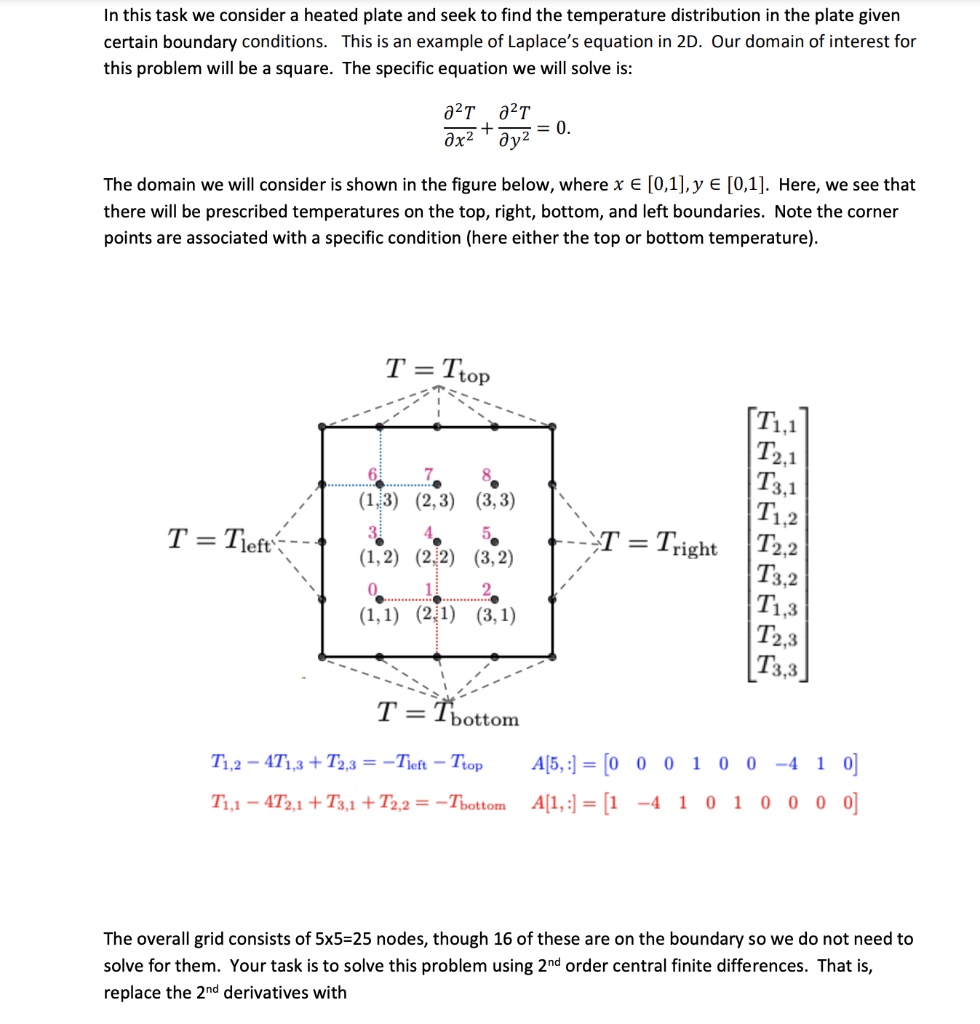
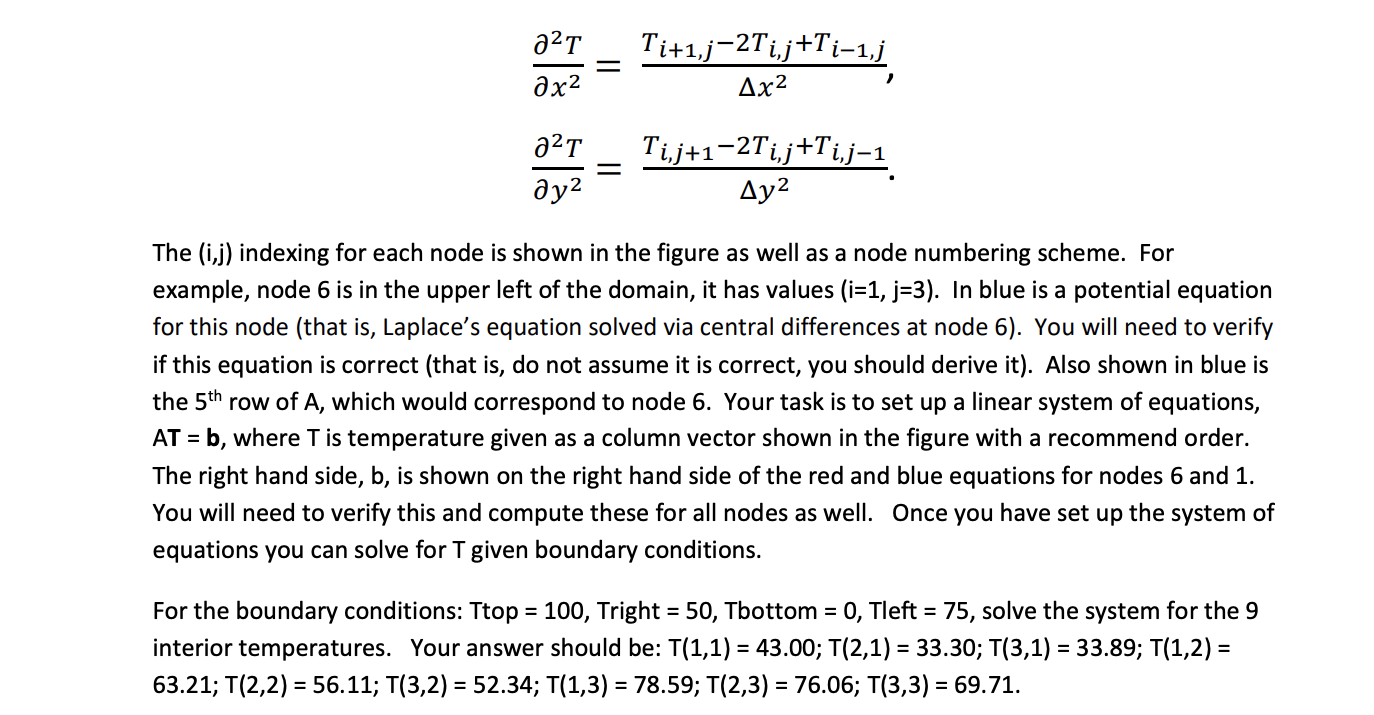
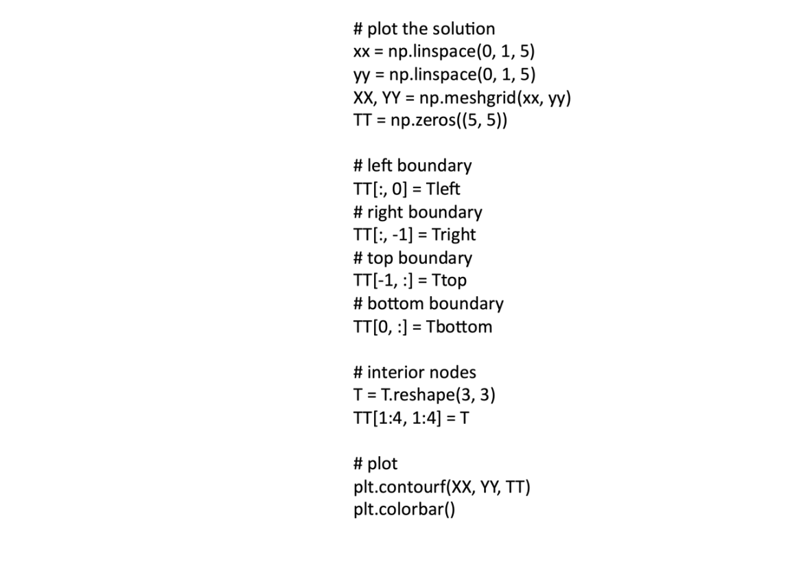
In this task we consider a heated plate and seek to find the temperature distribution in the plate given certain boundary conditions. This is an example of Laplace's equation in 2D. Our domain of interest for this problem will be a square. The specific equation we will solve is: x22T+y22T=0. The domain we will consider is shown in the figure below, where x[0,1],y[0,1]. Here, we see that there will be prescribed temperatures on the top, right, bottom, and left boundaries. Note the corner points are associated with a specific condition (here either the top or bottom temperature). T1,24T1,3+T2,3=TleftTtopA[5,:]=[000100410]T1,14T2,1+T3,1+T2,2=TbottomA[1,:]=[141010000] The overall grid consists of 55=25 nodes, though 16 of these are on the boundary so we do not need to solve for them. Your task is to solve this problem using 2nd order central finite differences. That is, replace the 2nd derivatives with x22T=x2Ti+1,j2Ti,j+Ti1,j,y22T=y2Ti,j+12Ti,j+Ti,j1. The (i,j) indexing for each node is shown in the figure as well as a node numbering scheme. For example, node 6 is in the upper left of the domain, it has values (i=1,j=3). In blue is a potential equation for this node (that is, Laplace's equation solved via central differences at node 6). You will need to verify if this equation is correct (that is, do not assume it is correct, you should derive it). Also shown in blue is the 5th row of A, which would correspond to node 6 . Your task is to set up a linear system of equations, AT=b, where T is temperature given as a column vector shown in the figure with a recommend order. The right hand side, b, is shown on the right hand side of the red and blue equations for nodes 6 and 1 . You will need to verify this and compute these for all nodes as well. Once you have set up the system of equations you can solve for T given boundary conditions. For the boundary conditions: Ttop =100, Tright =50, Tbottom =0, Tleft =75, solve the system for the 9 interior temperatures. Your answer should be: T(1,1)=43.00;T(2,1)=33.30;T(3,1)=33.89;T(1,2)= 63.21;T(2,2)=56.11;T(3,2)=52.34;T(1,3)=78.59;T(2,3)=76.06;T(3,3)=69.71 \# plot the solution xx=np.linspace(0,1,5)yy=np.linspace(0,1,5)XX,YY=np.meshgrid(xx,yy)TT=np.zeros((5,5)) \# left boundary TT[::0]=Tleft \# right boundary TT[:,1]= Tright \# top boundary TT [1,:]= Ttop \# bottom boundary TT[0, :] = Tbottom \# interior nodes T=T.reshape(3, 3) TT[1:4,1:4]=T \# plot plt.contourf(XX, YY, TT) plt.colorbar() Now, try a few different boundary conditions. For each case, provide a plot and the vector of T values. Case 1: Ttop =50, Tright =50, Tbottom =50, Tleft =50 Case 2: Ttop =50, Tright =50, Tbottom =50, Tleft =50 Case 2: Ttop =0, Tright =0, Tbottom =0, Tleft =100 Provide comments on each solution (generally related to if your results seem to make sense physically or not). Deliverables for this problem include your code saved as a5task2.py, your scratch work saved as a scanned pdf file named a5task2_scratch.pdf (there should be a lot of handwritten work for this problem as you sort out the governing equations in central difference form and how to get the code to work), and your results file saved as a5task2_results.pdf, which includes the plots, T vectors, and your brief thoughts on whether or not your results make sense. In this task we consider a heated plate and seek to find the temperature distribution in the plate given certain boundary conditions. This is an example of Laplace's equation in 2D. Our domain of interest for this problem will be a square. The specific equation we will solve is: x22T+y22T=0. The domain we will consider is shown in the figure below, where x[0,1],y[0,1]. Here, we see that there will be prescribed temperatures on the top, right, bottom, and left boundaries. Note the corner points are associated with a specific condition (here either the top or bottom temperature). T1,24T1,3+T2,3=TleftTtopA[5,:]=[000100410]T1,14T2,1+T3,1+T2,2=TbottomA[1,:]=[141010000] The overall grid consists of 55=25 nodes, though 16 of these are on the boundary so we do not need to solve for them. Your task is to solve this problem using 2nd order central finite differences. That is, replace the 2nd derivatives with x22T=x2Ti+1,j2Ti,j+Ti1,j,y22T=y2Ti,j+12Ti,j+Ti,j1. The (i,j) indexing for each node is shown in the figure as well as a node numbering scheme. For example, node 6 is in the upper left of the domain, it has values (i=1,j=3). In blue is a potential equation for this node (that is, Laplace's equation solved via central differences at node 6). You will need to verify if this equation is correct (that is, do not assume it is correct, you should derive it). Also shown in blue is the 5th row of A, which would correspond to node 6 . Your task is to set up a linear system of equations, AT=b, where T is temperature given as a column vector shown in the figure with a recommend order. The right hand side, b, is shown on the right hand side of the red and blue equations for nodes 6 and 1 . You will need to verify this and compute these for all nodes as well. Once you have set up the system of equations you can solve for T given boundary conditions. For the boundary conditions: Ttop =100, Tright =50, Tbottom =0, Tleft =75, solve the system for the 9 interior temperatures. Your answer should be: T(1,1)=43.00;T(2,1)=33.30;T(3,1)=33.89;T(1,2)= 63.21;T(2,2)=56.11;T(3,2)=52.34;T(1,3)=78.59;T(2,3)=76.06;T(3,3)=69.71 \# plot the solution xx=np.linspace(0,1,5)yy=np.linspace(0,1,5)XX,YY=np.meshgrid(xx,yy)TT=np.zeros((5,5)) \# left boundary TT[::0]=Tleft \# right boundary TT[:,1]= Tright \# top boundary TT [1,:]= Ttop \# bottom boundary TT[0, :] = Tbottom \# interior nodes T=T.reshape(3, 3) TT[1:4,1:4]=T \# plot plt.contourf(XX, YY, TT) plt.colorbar() Now, try a few different boundary conditions. For each case, provide a plot and the vector of T values. Case 1: Ttop =50, Tright =50, Tbottom =50, Tleft =50 Case 2: Ttop =50, Tright =50, Tbottom =50, Tleft =50 Case 2: Ttop =0, Tright =0, Tbottom =0, Tleft =100 Provide comments on each solution (generally related to if your results seem to make sense physically or not). Deliverables for this problem include your code saved as a5task2.py, your scratch work saved as a scanned pdf file named a5task2_scratch.pdf (there should be a lot of handwritten work for this problem as you sort out the governing equations in central difference form and how to get the code to work), and your results file saved as a5task2_results.pdf, which includes the plots, T vectors, and your brief thoughts on whether or not your results make sense