Instructions: Use the provided Live Script for your lab write$-$up$.$ Just like for all the other lab reports,

unless otherwise specified, include in your lab report all M$-$files, figures, MATLAB input commands, the

corresponding output, and the answers to the questions.

$($a$)$ Modify the function ex$\_($w$)$ith$\_(2)$eqs to solve the IVP $(4)$ for t using the MATLAB

routine ode$45.$ Call the new function LAB$04$ex$1.$

Let t$,$Y $($note the upper case Y $)$ be the output of ode$45$ and y and v the unknown functions.

Use the following commands to define the ODE:

function dYdt$=$f$($t$,$y$)$

y$=$Y$(1)$; v$=$Y$(2)$;

dYdt$=[$v;$8*$sin$($t$)-8*$v$-7*$y$]$;

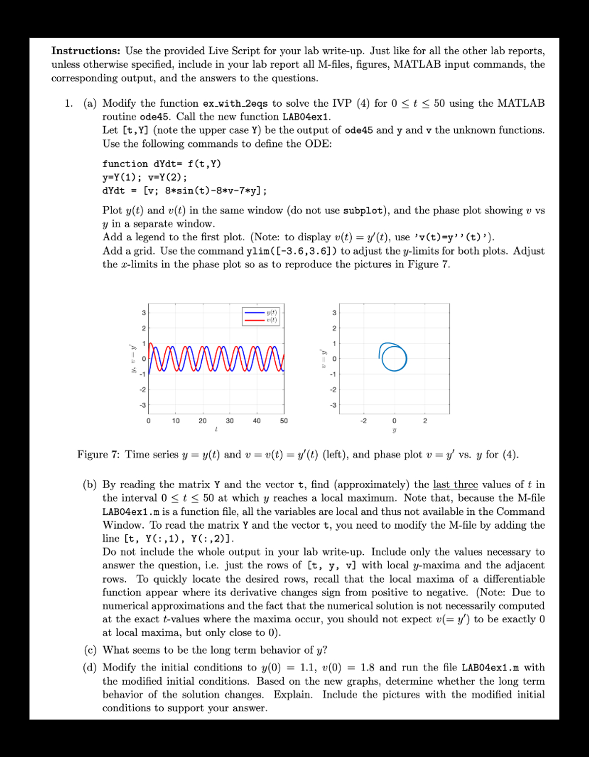
Plot y$($t$)$ and v$($t$)$ in the same window $($do not use subplot$),$ and the phase plot showing v vs

yv$($t$)=$y$^(\text{'})($t$),$ use $\text{'}$v $($t$)=$y $\text{'}\text{'}($t$)\text{'}[-3\mathrm{.}6,3\mathrm{.}6]$ to adjust the y$-$limits for both plots. Adjust

the x$-$limits in the phase plot so as to reproduce the pictures in Figure $7.$

Figure $7$: Time series y$=$y$($t$)$ and v$=$v$($t$)=$y$^(\text{'})($t$)($left$),$ and phase plot v$=$y$^(\text{'})$ vs$.$ y for $(4).$

$($b$)$ By reading the matrix Y and the vector t $,$ find $($approximately$)$ the last three values of t in

the interval t at which y reaches a local maximum. Note that, because the M$-$file

LAB$04$ex $1.$m is a function file, all the variables are local and thus not available in the Command

Window. To read the matrix Y and the vector t $,$ you need to modify the M $-$file by adding the

line t$,$Y$($:$,1),$Y$($:$,2)$y$,$v yt$-$values where the maxima occur, you should not expect v$(=$y$^(\text{'}))$ to be exactly $0$

at local maxima, but only close to $0$ y $?$

$($d$)$ Modify the initial conditions to y$(0)=1\mathrm{.}1,$v$(0)=1\mathrm{.}8$ and run the file LAB$04$ex$1.$m with

the modified initial conditions. Based on the new graphs, determine whether the long term

behavior of the solution changes. Explain. Include the pictures with the modified initial

conditions to support your answer.

ex$\_$with$\_$param

function ex$\_$with$\_$param

t$0=0$; tf $=3$; y$0=1$;

a $=1$;

$[$t$,$y$]=$ ode$45($@f$,[$t$0,$tf$],$y$0,[],$a$)$;

disp$([\text{'}$y$(\text{'}$ num$2$str$($t$($end$))\text{'})=\text{'}$ num$2$str$($y$($end$))])$

disp$([\text{'}$length of y $=\text{'}$ num$2$str$($length$($y$))])$

end

$\%-------------------------------------------------$

function dydt $=$ f$($t$,$y$,$a$)$

dydt $=-$a$*($y$-$exp$(-$t$))-$exp$(-$t$)$;

end

ex$\_$with$\_2$eqs

t$0=0$; tf $=20$; y$0=[10$;$60]$;

a $=\mathrm{.}8$; b $=\mathrm{.}01$; c $=\mathrm{.}6$; d $=\mathrm{.}1$;

$[$t$,$y$]=$ ode$45($@f$,[$t$0,$tf$],$y$0,[],$a$,$b$,$c$,$d$)$;

u$1=$ y$($:$,1)$; u$2=$ y$($:$,2)$; $\%$ y in output has $2$ columns corresponding to u$1$ and u$2$

figure$(1)$;

subplot$(2,1,1)$; plot$($t$,$u$1,\text{'}$b$-+\text{'})$; ylabel$(\text{'}$u$1\text{'})$;

subplot$(2,1,2)$; plot$($t$,$u$2,\text{'}$ro$-\text{'})$; ylabel$(\text{'}$u$2\text{'})$;

figure$(2)$

plot$($u$1,$u$2)$; axis square; xlabel$(\text{'}$u$\_1\text{'})$; ylabel$(\text{'}$u$\_2\text{'})$; $\%$ plot the phase plot

$\%----------------------------------------------------------------------$

function dydt $=$ f$($t$,$y$,$a$,$b$,$c$,$d$)$

u$1=$ y$(1)$; u$2=$ y$(2)$;

dydt $=[$ a$*$u$1-$b$*$u$1*$u$2$ ; $-$c$*$u$2+$d$*$u$1*$u$2]$;

end