Introduction

Microsoft Excel Pivot Tables are a quick and effective way to obtain various summary measurements about a dataset. It is then possible to use the Pivot Table results to calculate secondary measurements. In this tutorial, you will create a simple Pivot Table of frequency counts, and then use the results to calculate relative and percent frequencies.

The data has been collected in the Microsoft Excel Online file below. Open the spreadsheet and perform the required analysis to answer the questions below.

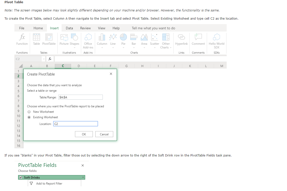
If you see "blanks" in your Pivot Table, filter those out by selecting the down arrow to the right of the Soft Drink row in the PivotTable Fields task pane.

PivotTable Fields

Choose fields:

Soft Drinks

$$Add to Report Filter If you see "blanks" in your Pivot Table, filter those out by selecting the down arrow to the right of the Soft Drink row in the PivotTable Fields task pane.

PivotTable Fields

Choose fields:

Soft Drinks

$\backslash ($

abla $\backslash )$ Add to Report Filter

III Add to Row Labels

$$ Add to Column Labels

$\backslash (\backslash$sum $\backslash )$ Add to Values

Add as Slicer

$\backslash (\backslash$mathrm$\{$A$\}\backslash$downarrow $\backslash )$ Sort Ascending

$\backslash (\backslash$mathrm$\{$Z$\}\backslash$downarrow $\backslash )$ Sort Descending

Sort By Value...

Clear Filter from 'Soft Drinks'

Label Filters

Value Filters

Filter...

Filter

Search Soft Drinks

Select item:

$($Select All$)$

Coca$-$Cola

Diet Coke

Dr$.$ Pepper

Mountain Dew

Pepsi

Sprite

$($blank$)$ Next, in the Pivot Table task pane, drag Soft Drinks to the Rows box and Values box. Make sure the Values box is set to Count of Soft Drinks. You now have created a Frequency Table.

$\backslash$begin$\{$tabular$\}\{$l$|$l$\}$

Drag fields between areas below: $\backslash \backslash$

$\backslash$begin$\{$tabular$\}\{|$l$|$l$\}$

$\backslash ($

abla $\backslash )$ & FILTERS

$\backslash$end$\{$tabular$\}$ & COLUMNS $\backslash \backslash$

$\backslash$hline

$\backslash$end$\{$tabular$\}$

In Column F and G$,$ create columns for "Relative Frequency" and "Percent Frequency $(\backslash \%)"$ that align with the Pivot Table headers.

In your new "Relative Frequency" and "Percent Frequency $(\backslash \%)"$ columns, proceed with those calculations so down the length of the Pivot Table and enter those values below.

$\backslash$begin$\{$tabular$\}\{$ll$\}$

Soft Drink & Frequency

$\backslash$end$\{$tabular$\}$ Coca$-$Cola

Diet Coke

Dr$.$ Pepper

Pepsi

Diet Coke

Coca$-$Cola

Coca$-$Cola

Sprite

Dr$.$ Pepper

Coca$-$Cola

Coca$-$Cola

Sprite

Sprite

Dr$.$ Pepper

Coca$-$Cola

Pepsi

Sprite

Diet Coke

Coca$-$Cola

Pepsi

Sprite

Mountain Dew

Pepsi

Diet Coke

Pepsi

Coca$-$Cola

Coca$-$Cola

Dr$.$ Pepper

Coca$-$Cola

Diet Coke

Sprite

Coca$-$Cola

Mountain Dew

Pepsi

Pepsi