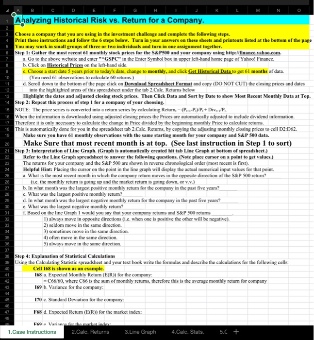
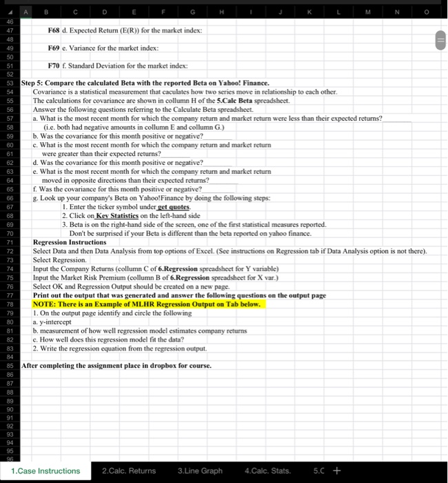
K L M N O I J Ahalyzing Historical Risk vs. Return for a Company. Choose a company that you are using in the investment challenge and complete the following steps. Print these instructions and follow the 6 steps below. Turn in your answers on these sheets and printouts listed at the bottom of the page You may work in small groups of three or two individuals and turn in one assignment together. Step 1: Gather the most recent 61 monthly stock prices for the S&P500 and your company using http://finance.yahoo.com. a. Go to the above website and enter "AGSPC" in the Enter Symbol box in upper left-hand home page of Yahoo! Finance. b. Click on Historical Prices on the left-hand side. c. Choose a start date 5 years prior to today's date, change to monthly, and click Get Historical Data to get 61 months of data. (You need l observations to calculate 60 returns.) d. Scroll down to the bottom of the page click on Download Spreadsheet Format and copy (DO NOT CUT) the closing prices and dates 12 into the highlighted areas of this spreadsheet under the tab 2.Calc. Returns below Highlight the dates and adjusted closing stock prices. Then Click Data and Sort by Date to show Most Recent Monthly Data at Top. 14 Step 2: Repeat this process of step 1 for a company of your choosing. 15 NOTE: The price series is converted into a retum series by calculating Return = P.-P.P+Dive/P 16 When the information is downloaded using adjusted closing prices the Prices are automatically adjusted to include dividend information. 17 Therefore it is only necessary to calculate the change in Price divided by the beginning monthly Price to calculate returns 18 This is automatically done for you in the spreadsheet tab 2.Calc. Returns, by copying the adjusting monthly closing prices to cell D2:D62. 19 Make sure you have 61 monthly observations with the same starting month for your company and S&P 500 data. 20 Make Sure that most recent month is at top. (See last instruction in Step 1 to sort) 21 Step 3: Interpretation of Line Graph. (Graph is automatically created hit tab Line Graph at bottom of spreadsheet.) Refer to the Line Graph spreadsheet to answer the following questions. (Note place cursor on a point to get values.) The returns for your company and the S&P 500 are shown in reverse chronological order (most recent is first). Helpful Hint: Placing the cursor on the point in the line graph will display the actual numerical input values for that point. a. What is the most recent month in which the company return moves in the opposite direction of the S&P 500 return? (ie, the monthly return is going up and the market return is going down, or v.v.) b. In what month was the largest positive monthly return for the company in the past five years? c. What was the largest positive monthly return? d. In what month was the largest negative monthly return for the company in the past five years? e. What was the largest negative monthly return? f. Based on the line Graph 1 would you say that your company retums and S&P 500 returns 1) always move in opposite directions (i.e. when one is positive the other will be negative). 2) seldom move in the same direction. 3) sometimes move in the same direction. 4) often move in the same direction. S) always move in the same direction. 38 Step 4: Explanation of Statistical Calculations 39 Using the Calculating Statistic spreadsheet and your text book write the formulas and describe the calculations for the following cells: Cell 168 is shown as an example. 168 a. Expected Monthly Retum (E(R)) for the company: -C66/60, where C66 is the sum of monthly returns, therefore this is the average monthly return for company 169 b. Variance for the company 170 c. Standard Deviation for the company: F68 d. Expected Return (E(R)) for the market index: F69 Variance for the marketindex 1.Case Instructions 2.Calc. Returns 3.Line Graph 4 .Calc. Stats. 5.C + A B C D E F G H I J K L M N O F68 d. Expected Return (E(R)) for the market index: F69 e. Variance for the market index: F70 f. Standard Deviation for the market index: 53 Step 5: Compare the calculated Beta with the reported Beta on Yahoo! Finance. Covariance is a statistical measurement that caculates how two series move in relationship to each other. The calculations for covariance are shown in collumn H of the 5.Calc Beta spreadsheet. Answer the following questions referring to the Calculate Beta spreadsheet. a. What is the most recent month for which the company return and market return were less than their expected retums? (i.c. both had negative amounts in collumn E and collumn G.) b. Was the covariance for this month positive or negative? e. What is the most recent month for which the company retum and market return were greater than their expected returns? d. Was the covariance for this month positive or negative? e. What is the most recent month for which the company retum and market return moved in opposite directions than their expected returns? f. Was the covariance for this month positive or negative? g. Look up your company's Beta on Yahoo!Finance by doing the following steps: 1. Enter the ticker symbol under get quotes 2. Click on Key Statistics on the left-hand side 3. Beta is on the right-hand side of the screen, one of the first statistical measures reported. Don't be surprised if your Beta is different than the beta reported on yahoo finance. Regression Instructions Select Data and then Data Analysis from top options of Excel. (See instructions on Regression tab if Data Analysis option is not there). Select Regression. Input the Company Returns (collumn C of 6.Regression spreadsheet for Y variable) Input the Market Risk Premium (collumn B of 6.Regression spreadsheet for X var.) Select OK and Regression Output should be created on a new page. Print out the output that was generated and answer the following questions on the output page NOTE: There is an example of MLHR Regression Output on Tab below. 1. On the output page identify and circle the following a. y-intercept b. measurement of how well regression model estimates company returns c. How well does this regression model fit the data? 2. Write the regression equation from the regression output. After completing the assignment place in dropbox for course. 1.Case Instructions 2. Calc. Returns 3.Line Graph 4.Calc. Stats. 5.C + ENNNNNNNN mor Date S&P 500 MSFT Mkt Returns Co. Returns Input Worksheet 1 5 /1/17 2381.73 67,69 -0.00103597 -0.0112474 in the highlighted column D copy a series of closing monthly 4/1/17 2384 2 68.46 0.009091209 0.03947765 prices for your company. This price series in collumn D is then 3/1/17 2362.72 65.86 -0.0003892 00293842 converted to a return series in column F. 2/1/17 2363 64 63 98 003719816 -0.01036353 5 1/1/17 2278 87 64 65 0.017884358 004039271 NOTE: You will cover MLHR data and the S&P 500 series is 12/1/16 2238 83 62 14 0.018200762 003119816 already done for you 11/1/16 2198.81 60.26 0.034174522 0.00567423 10/1/16 2126.15 59.92 -0.01942568 0.04027778 9/1/16 216827 57.6 -0.00123445 0.00243646 8/1/16 2170.95 57 46 -0.00121924 0.01376145 7/1/16 21736 56.68 0.035609801 0.10768032 6/1/16 2098.86 51.17 0.000910921 0.03452834 5/1/16 2096.95 5 3 0.015324602 006278321 4/1/16 20663 49.87 0.002699398 0.09704872 3/1/16 2059.74 55.23 0.065991115 008549526 2/1/16 1932 23 50.88 -0.00412836 -0.07642038 1/1/16 1940 24 55.09 -0.05073532 -0.00702956 12/1/15 2043 94 55 48 -001753019 002079121 11/1/15 2080.41 5435 0.000504869 003248478 10/1/15 2079 36 52 64 0 082983118 0 18933577 9/1/15 1920.03 44.26 002644283 0.01700363 8/1/15 1972 18 43.52 -0.06258082 -0.06809424 7/1/15 2103 84 46.7 0.01974203 0.05775762 6/1/15 2063 11 44.15 -0.02101167 -0.05783182 5/1/15 2107 39 46.85 0.010491382 -0.03659535 4/1/15 2085 51 48.64000852082 0.19626166 3/1/15 2067.89 40.86 -0.01739611 -0.07274796 2/1/15 2104.5 43.85 0.054892511 0.08539594 1/1/15 1994.99 40.4 0.03104081 0.13024755 12/1/14 2058.9 46.45 -0.00418859 -0.02844593 11/1/14 2067 56 47.81 0.024533589 0.01831736 10/1/14 2018.05 46.95 0.023201461 0.01272649 9/1/14 1972 29 46 36-001551384 0.02047108 8/1/14 2003 37 45.43 0.037655295 0 052595 7/1/14 1930 67 43.16 0.01507983 0.03501197 6/1/14 1960.23 41.7 0.019058332 0.0185638 5/1/14 1923.57 40.94 0.02103028 0.01336626 4/1/14 1883.95 40.4 0.006200789 -0.01439375 3/1/14 1872 34 40.99 0.006932166 0.06995565 2/1/14 1859 45 38.31 0.04311703 0.01242075 1/1/14 1782 5937 84 003558291 0.01149425 12/1/13 1848 36 37.41 0.023562792 010188828 11/1/13 1805 81 38.13 0.0280494720 07681449 10/1/13 1756.54 35.41 0.044595753 0.06400244 9/1/13 1681.55 33.28 0.029749523 -0.0035929 8/1/13 163297 33.4 -0.03129802 0.04899504 7/1/13 1685.73 31.84 0.04946208-007817026 6/1/13 1606 28 34 54 -00149993 -0.01031521 5/1/13 1630.74 349 0.020762812005438079 4/1/13 1597 57 331 0018085768 015693802 3/1/13 1569 19 28.61 0.035987724 002913676 2/1/13 1514.68 278 0.011060649 0.01275038 1/1/13 1498.11 27.45 0.050428097 0.02770505 12/1/12 1426 1926.71 0.00706823 0.0033B084 11/1/12 1416.18 26.62 0.002846717 -0.067274 10/1/12 1412.16 28.54 -001978941 -0.04099459 9/1/12 1440.67 29.76 0.024236154 -0.03439325 8/1/12 1406 58 30 82001976337 0.04580933 7/1/12 1379 32 29.47 0.012597574 -0.03661331 6/1/12 1362.16 30.59 0.039554982 0.04796159 61 5/1/12 1310.33 29.19 S SSR SONS 1. Case Instructions 2.Calc. Returns 3.Line Graph 4.Calc. Stats. 5.C + 1.Case Instructions 5/1/18 211/19 11/1/16 8/1/16 5/1/16 2.Calc. Returns 11/1/19 HET 15 3.Line Graph 2/1/15 Company vs. S&P 500 over time 16 8/10/10 MALAM 5/1/14 4.Calc. Stats. 21/141 CUIUS 5.C + 11/1/12 Co. Returns +Mt Returns This spreadsheet calculates the Expected Returns. Variances, and Standard Deviations of 2 Return Series Page down to bottom fow results Distance Market Company from Mean Variance(M) Variance Date Returns Returns R-ERR FIRER-ERREIRA May-17 0.00104 -0.01125 -0.01142 0.00013 Apr-17 000909 0.00MB -0.00129 0.00000 Nr.17 -0.00099 0.02208 -001077 0.00012 001347 000018 Feb-17 003720 - 0101022000200220COR Jan 17 0.01788 0.04009 0.00750 0.00005 Nov.16 0.03417 0.00567 Oct 16 901943 0062 0.023.79 -0.021 0.00089 0 02425 U-180035810.10208 0 .00001 0.00254 Apr-16 0.00270 -6.9705 0.01275 -0.00769 0.06661 0.00005 0.00309 Jan-16 -0.06074 -0.00703 -0.06112 0.00374 0.00010 0.00108 Sep-15 0.02544 0.01700 Aug-15 06258 -0.06809 0.09683 -007297 0.00138 0.00532 May 15 00 10-20-0000000011000000 0.00185 0.00000 000 0.00483 Feb-15 0.05489 0.08540 Jan-15 -0.00104 -0.13025 | | | | Nov.14 0.02453 0.01832 Od-14 0.02320 0.01273 Sep-14 -0.01551 0.02047 04451 0 04143 | | 0.01415 0.00199 0.00172 | | | 0.00020 0.00087 0.02547 0.00065 0.01909 Jul 14 00150B 0.03501 Jun-14 0.01905 0.01856 Apr 14 0.00620 -0.01439 0.01064 -0.00418 0.00011 0.00002 Feb-14 0.04312 0.01242 03273 0.00107 Dec-13 002350 Nov.13 0.02805 -0.01888 0. 001 0.01705 0 .00031 AL-13-00130 006900004168 00174 0 00109 0.01038 0.00011 May-13 0.02078 Apr 13 0.01809 0.05438 0.15594 Feb 13 0.01106 0.01275 0.00068 0.00000 . TUT | | | Od-12 001979 -0.04099 Sep-12 002424 -0.00439 - 03018 0 013850 2 .00019 -0.050.31 0.00253 -12 00:3935 004796 0.02917 0 00085 003204 0.00100 Market 0.00075 69 20 Variances Standard Deviation 1.Case Instructions 2.Calc. Returns 3.Line Graph 4.Calc. Stats. 5.C + This spreadsheet calculates the Covariance and Beta of a Company Return Series with a Mare Distance Market Company from Mean Date Returns Returns R-TIRI B Distance from Mean Covariance R AMBIRAN 0.01347 Mar 17 0.00030 0.02938 -0.01077 Feb 17 003720 -0.010360 02681 00040 0.11297 0.06958 Mary-16 001532 006276 Av. 16 000 000 Mar. 16 00650008550 Feb.15 -0.00413 07642 Jan-16 0,05074 0.00708 Dec.15 00175 002079 0 05561 -0.01451 0.06112 2 -0.02296 00014 0.01259 Sep-15 -9,02644 001700 Aug-15-000 -0009 OVET 0809 00606 00000 00012 Feb 15 005499 0.08540 0 04451 0.06048 Jan.15 -0.031040.13025 0.04143 0.14517 Dec 14 -0.00419002845 0.01457 0 No.54 002453 001832001455000940 Oct-14 007220001273004212 0 0919 Sep-54 -901551 002047 002500 0 00055 Aug-14 003766 005259 0 02727 003058 14 001508 003501 Jun-14 001906 001856 May-14 002103 001337 Apr-14 0.00620 -0.01439 Mar.14 0.00693 0.06096 Feb-14 0.04312 0.01242 Jan 14 -0.03558 0.01149 Dec 13 002356 091888 Nov.13 0.02805 0.07681 Oct-13 000 000 Sep-13 002973 -0.00059 Aug-13 -0.93130 004900 01322 Feb.13 001106 001275 000068 062314 095514 68 ER 69 Variance and Covariance 70 Standard Deviation 001039 0.00076 00371 0.00076 72 Calculating Beta Beta Covic M ar 1,00 74 Note: Beta measures the comovement of the company returns with the market ns 3 .Line Graph 4.Calc. Stats. 5.Calc. Beta 6.Regression MLHR + Assumes: 4.5% Annual Risk-free rate & 367% monthly Risk-free rate Regression Instructions Select Data & then Data Analysis from top Excel options (W Data Analysis option is not there see instructions below) Select Regression Input the Company Returns (column C of this spreadsheet for Y variable) Input the Market Risk Premium (column B of this spreadsheet for X var.) Select OK and Regression Output should be created on a new page Print out the output that was generated and answer the following questions on the output page. 1. On the output page identify and circle the following ay-intercept b. measurement of how well regression model estimates company returns c. How does this regression model fit the data? 2. Write the regression equation from the regression output. 16 Instructions for adding Regression option on Excel 1. Click the File on Top left and then click Options 2. Click Add-ins, and then in the Manage box, select Excel Add-ins. 3. Click Go. 4. In the Add-Ins available box, select the Analysis ToolPak check box, and then click OK Tip of Analysis ToolPak is not listed in the Add-Ins available box, click Browse to locate it. If you are prompted that the Analysis ToolPak is not currently installed on your computer, click Yes to install it 21 Met Returns Mit Premium Co. Retums -0.001035975 -0.004705975 -0.0112474 0.009091209 0.005421209 0.039477649 -0.000389197 -0.004059197 0029384198 0.03719816 0.03352816 -0.010363526 0.017884358 0.014214358 0.040392711 0.018200762 0.014530162 0031198159 0.034 174522 0030504522 0005674232 -0.019425679 -0.023095679 0.040277779 -0.001234451 -0.004904451 0.00243546 -0.001219243 -0.004889243 0.01376145 0035609801 0.031939801 0.101680325 0.000910921 0.002759079 -0.03452834 0.015324002 0.011654602 0.062763206 0.002699398 -0.000970602 -0,097048724 0.065991115 0.062321115 0085495252 -0.00412836 -0.00779836 -0.075420385 -0.050735322 -0.054405322 -0.00702956 -0.017530185 -0.021200185 0.020791206 0.000504869 -0.003165131 0.032484784 0.082983118 0.079313118 0.189335774 -0.026442832 -0.030112832 0.017003631 -0.062580818 -0,066250818 -0.068094238 0.01974203 0.01607203 0.057757619 -0.021011672 -0.024681672 -0.057831817 0.010491382 0.006821382 -0.036595354 0.00852082 0.00485082 0.196261658 -0.017396107 -0.021056107 -0.072747962 0.054892511 0.051222511 0.085395936 -0.031040805 -0.034710806 -0.130247554 -0.004188588 -0.007858588 -0.028445931 0.024533589 0.020863599 0.018317359 0.023201461 0.019531461 0.012726488 -0.015513837 -0.019183837 0020471076 0.037655295 0.033985295 0.0525044995 -0.015079831 -0.019749831 0.035011966 0.019058332 0.015388332 001856-3801 0.02103028 0.01736028 0.013366262 0.006200789 0.002530789 -0.014393754 0.006932166 0.003262166 0.069965649 0.04311703 0.03944703 0.012420745 -0035582906 -0.039252906 0011494253 0.023562792 0.019892792 -0.018382795 0.028049472 0.024379472 0.076814487 0.044595753 0.040925753 0064002436 0.0297495230025079523 -0.003592904 -0.031298019 -0.03496B019 0.048995038 0.04946208 0.04579208 -0.078170264 -0014999002 -0.018669302 -0.010315214 0.020762812 0017092812 0054380789 0.018085768 0.014415768 0.156938023 0.035997724 0.002317724 0.029136764 0.011050649 0.007390649 0.012750382 0.050428097 0046758097 0027705055 0.00706823 0.00339823 0.003380841 0.002846717 -0.000823283 -0.067273999 -0.01978941 -0.02345941 -0.04099459 0.024236154 0.020566154 -0.034393251 0.01976337 0.01609337 0.045809333 0.012597574 0008927574 -0.036613305 0.039554982 0.035884982 0047961595 40 42 44 47 54 61 3.Line Graph 4.Calc. Stats. 5.Calc. Beta 6.Regression MLAR + F G H This page is an example of the regression output generated for the MLHR data. SUMMARY OUTPUT 2 5 6 7 8 9 Regression Statistics Multiple R 0.2943897 R Square 0.0866653 Adjusted R Square 0.0709181 Goodness of Fit Measurement Standard Error 0.0800974 Observations 60 10 df 1 0 11 ANOVA 12 13 Regression 14 Residual 15 Total 16 58 59 SS M SF Significance F .035308545 0.03531 5.50355 0.022417617 0.372104303 0.00642 0.407412848 18 19 Intercept X Variable 1 Coefficients 0.0058013 .8629369 Standard Error 0 .010340535 0.367838762 StatP -value Lower 95% Upper 95% Lower 95.0% 0.56103 0.57694 -0.014897513 0.02650015 -0.014897513 2.34597 0.02242 0.126627647 1.5992462 0.126627647 Upper 95.0% 0.026500146 1.599246198 0 22 Regression Equation: Y = 0.0058013 + 0.8629X K L M N O I J Ahalyzing Historical Risk vs. Return for a Company. Choose a company that you are using in the investment challenge and complete the following steps. Print these instructions and follow the 6 steps below. Turn in your answers on these sheets and printouts listed at the bottom of the page You may work in small groups of three or two individuals and turn in one assignment together. Step 1: Gather the most recent 61 monthly stock prices for the S&P500 and your company using http://finance.yahoo.com. a. Go to the above website and enter "AGSPC" in the Enter Symbol box in upper left-hand home page of Yahoo! Finance. b. Click on Historical Prices on the left-hand side. c. Choose a start date 5 years prior to today's date, change to monthly, and click Get Historical Data to get 61 months of data. (You need l observations to calculate 60 returns.) d. Scroll down to the bottom of the page click on Download Spreadsheet Format and copy (DO NOT CUT) the closing prices and dates 12 into the highlighted areas of this spreadsheet under the tab 2.Calc. Returns below Highlight the dates and adjusted closing stock prices. Then Click Data and Sort by Date to show Most Recent Monthly Data at Top. 14 Step 2: Repeat this process of step 1 for a company of your choosing. 15 NOTE: The price series is converted into a retum series by calculating Return = P.-P.P+Dive/P 16 When the information is downloaded using adjusted closing prices the Prices are automatically adjusted to include dividend information. 17 Therefore it is only necessary to calculate the change in Price divided by the beginning monthly Price to calculate returns 18 This is automatically done for you in the spreadsheet tab 2.Calc. Returns, by copying the adjusting monthly closing prices to cell D2:D62. 19 Make sure you have 61 monthly observations with the same starting month for your company and S&P 500 data. 20 Make Sure that most recent month is at top. (See last instruction in Step 1 to sort) 21 Step 3: Interpretation of Line Graph. (Graph is automatically created hit tab Line Graph at bottom of spreadsheet.) Refer to the Line Graph spreadsheet to answer the following questions. (Note place cursor on a point to get values.) The returns for your company and the S&P 500 are shown in reverse chronological order (most recent is first). Helpful Hint: Placing the cursor on the point in the line graph will display the actual numerical input values for that point. a. What is the most recent month in which the company return moves in the opposite direction of the S&P 500 return? (ie, the monthly return is going up and the market return is going down, or v.v.) b. In what month was the largest positive monthly return for the company in the past five years? c. What was the largest positive monthly return? d. In what month was the largest negative monthly return for the company in the past five years? e. What was the largest negative monthly return? f. Based on the line Graph 1 would you say that your company retums and S&P 500 returns 1) always move in opposite directions (i.e. when one is positive the other will be negative). 2) seldom move in the same direction. 3) sometimes move in the same direction. 4) often move in the same direction. S) always move in the same direction. 38 Step 4: Explanation of Statistical Calculations 39 Using the Calculating Statistic spreadsheet and your text book write the formulas and describe the calculations for the following cells: Cell 168 is shown as an example. 168 a. Expected Monthly Retum (E(R)) for the company: -C66/60, where C66 is the sum of monthly returns, therefore this is the average monthly return for company 169 b. Variance for the company 170 c. Standard Deviation for the company: F68 d. Expected Return (E(R)) for the market index: F69 Variance for the marketindex 1.Case Instructions 2.Calc. Returns 3.Line Graph 4 .Calc. Stats. 5.C + A B C D E F G H I J K L M N O F68 d. Expected Return (E(R)) for the market index: F69 e. Variance for the market index: F70 f. Standard Deviation for the market index: 53 Step 5: Compare the calculated Beta with the reported Beta on Yahoo! Finance. Covariance is a statistical measurement that caculates how two series move in relationship to each other. The calculations for covariance are shown in collumn H of the 5.Calc Beta spreadsheet. Answer the following questions referring to the Calculate Beta spreadsheet. a. What is the most recent month for which the company return and market return were less than their expected retums? (i.c. both had negative amounts in collumn E and collumn G.) b. Was the covariance for this month positive or negative? e. What is the most recent month for which the company retum and market return were greater than their expected returns? d. Was the covariance for this month positive or negative? e. What is the most recent month for which the company retum and market return moved in opposite directions than their expected returns? f. Was the covariance for this month positive or negative? g. Look up your company's Beta on Yahoo!Finance by doing the following steps: 1. Enter the ticker symbol under get quotes 2. Click on Key Statistics on the left-hand side 3. Beta is on the right-hand side of the screen, one of the first statistical measures reported. Don't be surprised if your Beta is different than the beta reported on yahoo finance. Regression Instructions Select Data and then Data Analysis from top options of Excel. (See instructions on Regression tab if Data Analysis option is not there). Select Regression. Input the Company Returns (collumn C of 6.Regression spreadsheet for Y variable) Input the Market Risk Premium (collumn B of 6.Regression spreadsheet for X var.) Select OK and Regression Output should be created on a new page. Print out the output that was generated and answer the following questions on the output page NOTE: There is an example of MLHR Regression Output on Tab below. 1. On the output page identify and circle the following a. y-intercept b. measurement of how well regression model estimates company returns c. How well does this regression model fit the data? 2. Write the regression equation from the regression output. After completing the assignment place in dropbox for course. 1.Case Instructions 2. Calc. Returns 3.Line Graph 4.Calc. Stats. 5.C + ENNNNNNNN mor Date S&P 500 MSFT Mkt Returns Co. Returns Input Worksheet 1 5 /1/17 2381.73 67,69 -0.00103597 -0.0112474 in the highlighted column D copy a series of closing monthly 4/1/17 2384 2 68.46 0.009091209 0.03947765 prices for your company. This price series in collumn D is then 3/1/17 2362.72 65.86 -0.0003892 00293842 converted to a return series in column F. 2/1/17 2363 64 63 98 003719816 -0.01036353 5 1/1/17 2278 87 64 65 0.017884358 004039271 NOTE: You will cover MLHR data and the S&P 500 series is 12/1/16 2238 83 62 14 0.018200762 003119816 already done for you 11/1/16 2198.81 60.26 0.034174522 0.00567423 10/1/16 2126.15 59.92 -0.01942568 0.04027778 9/1/16 216827 57.6 -0.00123445 0.00243646 8/1/16 2170.95 57 46 -0.00121924 0.01376145 7/1/16 21736 56.68 0.035609801 0.10768032 6/1/16 2098.86 51.17 0.000910921 0.03452834 5/1/16 2096.95 5 3 0.015324602 006278321 4/1/16 20663 49.87 0.002699398 0.09704872 3/1/16 2059.74 55.23 0.065991115 008549526 2/1/16 1932 23 50.88 -0.00412836 -0.07642038 1/1/16 1940 24 55.09 -0.05073532 -0.00702956 12/1/15 2043 94 55 48 -001753019 002079121 11/1/15 2080.41 5435 0.000504869 003248478 10/1/15 2079 36 52 64 0 082983118 0 18933577 9/1/15 1920.03 44.26 002644283 0.01700363 8/1/15 1972 18 43.52 -0.06258082 -0.06809424 7/1/15 2103 84 46.7 0.01974203 0.05775762 6/1/15 2063 11 44.15 -0.02101167 -0.05783182 5/1/15 2107 39 46.85 0.010491382 -0.03659535 4/1/15 2085 51 48.64000852082 0.19626166 3/1/15 2067.89 40.86 -0.01739611 -0.07274796 2/1/15 2104.5 43.85 0.054892511 0.08539594 1/1/15 1994.99 40.4 0.03104081 0.13024755 12/1/14 2058.9 46.45 -0.00418859 -0.02844593 11/1/14 2067 56 47.81 0.024533589 0.01831736 10/1/14 2018.05 46.95 0.023201461 0.01272649 9/1/14 1972 29 46 36-001551384 0.02047108 8/1/14 2003 37 45.43 0.037655295 0 052595 7/1/14 1930 67 43.16 0.01507983 0.03501197 6/1/14 1960.23 41.7 0.019058332 0.0185638 5/1/14 1923.57 40.94 0.02103028 0.01336626 4/1/14 1883.95 40.4 0.006200789 -0.01439375 3/1/14 1872 34 40.99 0.006932166 0.06995565 2/1/14 1859 45 38.31 0.04311703 0.01242075 1/1/14 1782 5937 84 003558291 0.01149425 12/1/13 1848 36 37.41 0.023562792 010188828 11/1/13 1805 81 38.13 0.0280494720 07681449 10/1/13 1756.54 35.41 0.044595753 0.06400244 9/1/13 1681.55 33.28 0.029749523 -0.0035929 8/1/13 163297 33.4 -0.03129802 0.04899504 7/1/13 1685.73 31.84 0.04946208-007817026 6/1/13 1606 28 34 54 -00149993 -0.01031521 5/1/13 1630.74 349 0.020762812005438079 4/1/13 1597 57 331 0018085768 015693802 3/1/13 1569 19 28.61 0.035987724 002913676 2/1/13 1514.68 278 0.011060649 0.01275038 1/1/13 1498.11 27.45 0.050428097 0.02770505 12/1/12 1426 1926.71 0.00706823 0.0033B084 11/1/12 1416.18 26.62 0.002846717 -0.067274 10/1/12 1412.16 28.54 -001978941 -0.04099459 9/1/12 1440.67 29.76 0.024236154 -0.03439325 8/1/12 1406 58 30 82001976337 0.04580933 7/1/12 1379 32 29.47 0.012597574 -0.03661331 6/1/12 1362.16 30.59 0.039554982 0.04796159 61 5/1/12 1310.33 29.19 S SSR SONS 1. Case Instructions 2.Calc. Returns 3.Line Graph 4.Calc. Stats. 5.C + 1.Case Instructions 5/1/18 211/19 11/1/16 8/1/16 5/1/16 2.Calc. Returns 11/1/19 HET 15 3.Line Graph 2/1/15 Company vs. S&P 500 over time 16 8/10/10 MALAM 5/1/14 4.Calc. Stats. 21/141 CUIUS 5.C + 11/1/12 Co. Returns +Mt Returns This spreadsheet calculates the Expected Returns. Variances, and Standard Deviations of 2 Return Series Page down to bottom fow results Distance Market Company from Mean Variance(M) Variance Date Returns Returns R-ERR FIRER-ERREIRA May-17 0.00104 -0.01125 -0.01142 0.00013 Apr-17 000909 0.00MB -0.00129 0.00000 Nr.17 -0.00099 0.02208 -001077 0.00012 001347 000018 Feb-17 003720 - 0101022000200220COR Jan 17 0.01788 0.04009 0.00750 0.00005 Nov.16 0.03417 0.00567 Oct 16 901943 0062 0.023.79 -0.021 0.00089 0 02425 U-180035810.10208 0 .00001 0.00254 Apr-16 0.00270 -6.9705 0.01275 -0.00769 0.06661 0.00005 0.00309 Jan-16 -0.06074 -0.00703 -0.06112 0.00374 0.00010 0.00108 Sep-15 0.02544 0.01700 Aug-15 06258 -0.06809 0.09683 -007297 0.00138 0.00532 May 15 00 10-20-0000000011000000 0.00185 0.00000 000 0.00483 Feb-15 0.05489 0.08540 Jan-15 -0.00104 -0.13025 | | | | Nov.14 0.02453 0.01832 Od-14 0.02320 0.01273 Sep-14 -0.01551 0.02047 04451 0 04143 | | 0.01415 0.00199 0.00172 | | | 0.00020 0.00087 0.02547 0.00065 0.01909 Jul 14 00150B 0.03501 Jun-14 0.01905 0.01856 Apr 14 0.00620 -0.01439 0.01064 -0.00418 0.00011 0.00002 Feb-14 0.04312 0.01242 03273 0.00107 Dec-13 002350 Nov.13 0.02805 -0.01888 0. 001 0.01705 0 .00031 AL-13-00130 006900004168 00174 0 00109 0.01038 0.00011 May-13 0.02078 Apr 13 0.01809 0.05438 0.15594 Feb 13 0.01106 0.01275 0.00068 0.00000 . TUT | | | Od-12 001979 -0.04099 Sep-12 002424 -0.00439 - 03018 0 013850 2 .00019 -0.050.31 0.00253 -12 00:3935 004796 0.02917 0 00085 003204 0.00100 Market 0.00075 69 20 Variances Standard Deviation 1.Case Instructions 2.Calc. Returns 3.Line Graph 4.Calc. Stats. 5.C + This spreadsheet calculates the Covariance and Beta of a Company Return Series with a Mare Distance Market Company from Mean Date Returns Returns R-TIRI B Distance from Mean Covariance R AMBIRAN 0.01347 Mar 17 0.00030 0.02938 -0.01077 Feb 17 003720 -0.010360 02681 00040 0.11297 0.06958 Mary-16 001532 006276 Av. 16 000 000 Mar. 16 00650008550 Feb.15 -0.00413 07642 Jan-16 0,05074 0.00708 Dec.15 00175 002079 0 05561 -0.01451 0.06112 2 -0.02296 00014 0.01259 Sep-15 -9,02644 001700 Aug-15-000 -0009 OVET 0809 00606 00000 00012 Feb 15 005499 0.08540 0 04451 0.06048 Jan.15 -0.031040.13025 0.04143 0.14517 Dec 14 -0.00419002845 0.01457 0 No.54 002453 001832001455000940 Oct-14 007220001273004212 0 0919 Sep-54 -901551 002047 002500 0 00055 Aug-14 003766 005259 0 02727 003058 14 001508 003501 Jun-14 001906 001856 May-14 002103 001337 Apr-14 0.00620 -0.01439 Mar.14 0.00693 0.06096 Feb-14 0.04312 0.01242 Jan 14 -0.03558 0.01149 Dec 13 002356 091888 Nov.13 0.02805 0.07681 Oct-13 000 000 Sep-13 002973 -0.00059 Aug-13 -0.93130 004900 01322 Feb.13 001106 001275 000068 062314 095514 68 ER 69 Variance and Covariance 70 Standard Deviation 001039 0.00076 00371 0.00076 72 Calculating Beta Beta Covic M ar 1,00 74 Note: Beta measures the comovement of the company returns with the market ns 3 .Line Graph 4.Calc. Stats. 5.Calc. Beta 6.Regression MLHR + Assumes: 4.5% Annual Risk-free rate & 367% monthly Risk-free rate Regression Instructions Select Data & then Data Analysis from top Excel options (W Data Analysis option is not there see instructions below) Select Regression Input the Company Returns (column C of this spreadsheet for Y variable) Input the Market Risk Premium (column B of this spreadsheet for X var.) Select OK and Regression Output should be created on a new page Print out the output that was generated and answer the following questions on the output page. 1. On the output page identify and circle the following ay-intercept b. measurement of how well regression model estimates company returns c. How does this regression model fit the data? 2. Write the regression equation from the regression output. 16 Instructions for adding Regression option on Excel 1. Click the File on Top left and then click Options 2. Click Add-ins, and then in the Manage box, select Excel Add-ins. 3. Click Go. 4. In the Add-Ins available box, select the Analysis ToolPak check box, and then click OK Tip of Analysis ToolPak is not listed in the Add-Ins available box, click Browse to locate it. If you are prompted that the Analysis ToolPak is not currently installed on your computer, click Yes to install it 21 Met Returns Mit Premium Co. Retums -0.001035975 -0.004705975 -0.0112474 0.009091209 0.005421209 0.039477649 -0.000389197 -0.004059197 0029384198 0.03719816 0.03352816 -0.010363526 0.017884358 0.014214358 0.040392711 0.018200762 0.014530162 0031198159 0.034 174522 0030504522 0005674232 -0.019425679 -0.023095679 0.040277779 -0.001234451 -0.004904451 0.00243546 -0.001219243 -0.004889243 0.01376145 0035609801 0.031939801 0.101680325 0.000910921 0.002759079 -0.03452834 0.015324002 0.011654602 0.062763206 0.002699398 -0.000970602 -0,097048724 0.065991115 0.062321115 0085495252 -0.00412836 -0.00779836 -0.075420385 -0.050735322 -0.054405322 -0.00702956 -0.017530185 -0.021200185 0.020791206 0.000504869 -0.003165131 0.032484784 0.082983118 0.079313118 0.189335774 -0.026442832 -0.030112832 0.017003631 -0.062580818 -0,066250818 -0.068094238 0.01974203 0.01607203 0.057757619 -0.021011672 -0.024681672 -0.057831817 0.010491382 0.006821382 -0.036595354 0.00852082 0.00485082 0.196261658 -0.017396107 -0.021056107 -0.072747962 0.054892511 0.051222511 0.085395936 -0.031040805 -0.034710806 -0.130247554 -0.004188588 -0.007858588 -0.028445931 0.024533589 0.020863599 0.018317359 0.023201461 0.019531461 0.012726488 -0.015513837 -0.019183837 0020471076 0.037655295 0.033985295 0.0525044995 -0.015079831 -0.019749831 0.035011966 0.019058332 0.015388332 001856-3801 0.02103028 0.01736028 0.013366262 0.006200789 0.002530789 -0.014393754 0.006932166 0.003262166 0.069965649 0.04311703 0.03944703 0.012420745 -0035582906 -0.039252906 0011494253 0.023562792 0.019892792 -0.018382795 0.028049472 0.024379472 0.076814487 0.044595753 0.040925753 0064002436 0.0297495230025079523 -0.003592904 -0.031298019 -0.03496B019 0.048995038 0.04946208 0.04579208 -0.078170264 -0014999002 -0.018669302 -0.010315214 0.020762812 0017092812 0054380789 0.018085768 0.014415768 0.156938023 0.035997724 0.002317724 0.029136764 0.011050649 0.007390649 0.012750382 0.050428097 0046758097 0027705055 0.00706823 0.00339823 0.003380841 0.002846717 -0.000823283 -0.067273999 -0.01978941 -0.02345941 -0.04099459 0.024236154 0.020566154 -0.034393251 0.01976337 0.01609337 0.045809333 0.012597574 0008927574 -0.036613305 0.039554982 0.035884982 0047961595 40 42 44 47 54 61 3.Line Graph 4.Calc. Stats. 5.Calc. Beta 6.Regression MLAR + F G H This page is an example of the regression output generated for the MLHR data. SUMMARY OUTPUT 2 5 6 7 8 9 Regression Statistics Multiple R 0.2943897 R Square 0.0866653 Adjusted R Square 0.0709181 Goodness of Fit Measurement Standard Error 0.0800974 Observations 60 10 df 1 0 11 ANOVA 12 13 Regression 14 Residual 15 Total 16 58 59 SS M SF Significance F .035308545 0.03531 5.50355 0.022417617 0.372104303 0.00642 0.407412848 18 19 Intercept X Variable 1 Coefficients 0.0058013 .8629369 Standard Error 0 .010340535 0.367838762 StatP -value Lower 95% Upper 95% Lower 95.0% 0.56103 0.57694 -0.014897513 0.02650015 -0.014897513 2.34597 0.02242 0.126627647 1.5992462 0.126627647 Upper 95.0% 0.026500146 1.599246198 0 22 Regression Equation: Y = 0.0058013 + 0.8629X