.... Kindly help me understand this problems only

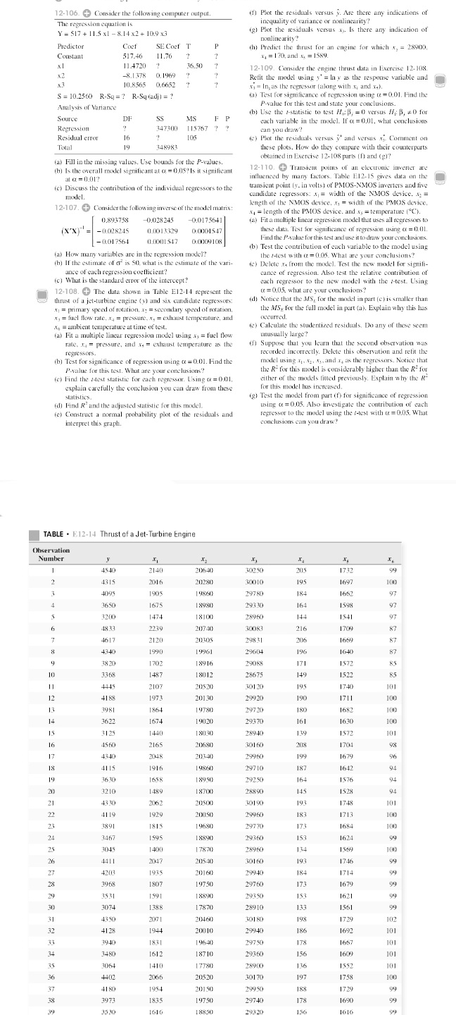
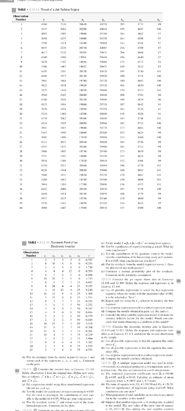
12-106. + Consider the following computer output. (f) Plot the residuals versus y. Are there any indications of The regression equation is inequality of variance or nonlinearity? Y = 517 + 11.5 xl - 8.14 x2+ 10.9 x3 (2) Plot the residuals versus a;. Is there any indication of nonlinearity? Predictor Coof SE Coof T (h) Predict the thrust for an engine for which x, = 28900. Constant 517.46 11.76 1, = 170, and x, = 1589. 11.4720 ? 36.50 12-109. Consider the engine thrust data in Exercise 12-108. -8.1378 0. 1969 Refit the model using y' = In y as the response variable and 10.8565 0.6652 vy= In, as the regressor (along with N, and x,). $ = 10.2560 R-Sq =? R-Squadj) = ? (a) Test for significance of regression using o =0.01. Find the Analysis of Variance P-value for this test and state your conclusions. (b) Use the /-statistic to test Ho: B, =0 versus H B, 20 for Source DF SS MS P each variable in the model. If o = 0.01. what conclusions Regression 347300 115767 9 can you draw? Residual error 16 10 (e) Plot the residuals versus y' and versus xy Comment on Total 348983 these plots. How do they compare with their counterparts (as Fill in the missing values. Use bounds for the P-values. obtained in Exercise 12-108 parts (f) and (g)? bj Is the overall model significant at o = 0.05 Is it significant 12-110. + Trunsiem points of an electronic inverter are at a = 0.017 influenced by many factors. Table E12-15 gives data on the (c) Discuss the contribution of the individual regressors to the transient point (y. in volts) of PMOS-NMOS inverters and five model. candidate regressors: * = width of the NMOS device. *; = 12-107. + Consider the following inverse of the model matrix: length of the NMOS device, x, = width of the PMOS device. * = length of the PMOS device, and x5 = temperature ["C). 0.893758 -0.028245 -0.0175641 (a) Fit a multiple linear regression model that uses all regressones to (x'X) = -0.028245 0.0013329 0.0001547 these data. Test for significance of regression using ( = 0.01. -0.017564 0.0001 547 0.0909 108 Find the P-value for this test and use it to draw your conclusions. (b) Test the contribution of each variable to the model using (a) How many variables are in the regression model? the rest with o =0.05. What are your conclusions? hi If the estimate of ' is 50. what is the estimate of the vari- () Delete x. from the model. Test the new model for signifi- ance of cach regression cocfficient? cance of regression. Also test the relative contribution of (c) What is the standard error of the intercept?" each regressor to the new model with the /-test. Using 12-108. + The data shown in Table E1 2-14 represent the D =0.05. what are your conclusions? thrust of a jet-turbine engine ()) and six candidate regressors. (d) Notice that the MS, for the model in part (c) is smaller than = primary speed of rotation, I = secondary speed of rotation, the MS, for the full model in part (a). Explain why this has = fuel flow rate. I. = pressure, x, = exhaust temperature, and occurred. " = ambient temperature at time of test. () Calculate the studentized residuals. Do any of these seem (@) Fit a multiple linear regression model using *, = fuel flow unusually large? rate. I. = pressure, and x, = exhaust temperature as the (f) Suppose that you learn that the second observation was regressors. recorded incorrectly. Delete this observation and refit the (b) Test for significance of regression using o =0.01. Find the model using 1, $2, $1, and r, as the regressors. Notice that P.value for this test. What are your conclusions? the R- for this model is considerably higher than the R for (e) Find the zest statistic for each regressor. Using of =0.01, either of the models fitted previously. Explain why the R- explain carefully the conclusion you can draw from these for this model has increased. statistics. (2) Test the model from part (f) for significance of regression (d) Find R and the adjusted statistic for this model. using 0 =0.05. Also investigate the contribution of each (e) Construct a normal probability plot of the residuals and regressor to the model using the f-test with o = 0.05. What interpret this graph. conclusions can you draw? TABLE . E12-14 Thrust of a Jet-Turbine Engine Observation Number 4540 2140 20640 30250 205 1732 99 4315 2016 20280 30010 195 1697 100 4095 1905 19860 297 80 184 1662 97 365( 1675 18980 293 30 164 1598 97 3240 1474 18100 28960 144 1541 97 6 1833 2239 20740 30083 216 1709 87 4617 21201 20305 298 31 206 1669 87 OF Et 1990 19961 29604 196 1640 87 38 20 1702 18916 29088 171 1572 85 3368 1487 18012 28675 149 1522 85 4445 2107 20520 301 20 195 1740 101 41 88 197: 20130 29920 190 1711 100 3981 1864 19780 29720 180 1682 100 3622 1674 19020 293 70 161 1630 100 3125 1440 18030 OF 682 139 1572 101 4560 2165 20680 30160 208 1704 98 4340 20340 29960 199 1679 96 41 15 1916 19860 29710 187 1642 94 363 1658 18950 29250 164 1576 94 20 3210 1489 18300 28890 145 1528 94 21 43 30 2062 20500 30190 193 1748 101 22 41 19 1929 20050 29960 183 1713 100 3891 1815 19680 297 70 173 1684 100 24 3467 1595 18890 29360 153 1624 99 25 3045 1400 17870 28960 134 1569 100 26 4411 2047 20540 30160 193 1746 99 42013 193 20160 29940 184 1714 99 3968 1807 19750 29760 173 1679 99 3531 1591 18890 29350 153 1621 99 3074 1388 17870 28910 133 1561 99 4350 207 1 20460 301 80 198 1729 102 41 28 194 20010 29940 186 1692 101 3940 1831 19640 297 50 178 1667 101 3480 1612 18710 29360 156 1609 101 3064 1410 17780 28900 136 1552 101 4402 2066 20520 301 70 197 1758 100 41 80 1954 20150 299 50 188 1729 49 3973 1835 19750 29740 178 1690 99TABLE . E12-14 Thrust of a Jet-Turbine Engine Observation Number 4540 2140 20640 30250 205 1732 99 4315 2016 20280 30010 195 1697 100 1095 1905 19860 297 80) 184 1662 97 3650 1675 1 8980 293 30 164 159% 97 324X 1474 18100 28960 144 1541 97 4833 2239 20740 30083 216 1709 4617 2120 20305 29831 206 1669 43-40 1990 19961 29604 196 1640 87 38 20 1702 18916 2908 131 1572 336 1487 18012 28675 149 1522 85 4145 2107 20520 301 20) 195 1740 101 41 88 197 3 20130 29920 190 1711 100 3981 1864 19780 297 20 180 1682 100 14 3622 1674 19020 293 70 161 1630 100 15 3125 1440 18030 28940 139 1572 101 4560 2165 20680 30160 208 1704 98 4340 20)48 20340 29460 199 1679 96 18 41 15 1916 19860 297 10 187 1642 94 19 36.3 1658 18950 29250 164 1576 94 20 32 10 1489 18700 28890 145 1528 94 43 3 2062 20500 30190 193 1748 101 41 19 1929 20050 29960 183 1713 100 23 3891 1815 19680 297 70 133 1684 100 24 3467 1595 18890 29360 153 1624 99 25 3045 1400 17870 28960 134 1569 100 4411 2047 20540 30160 193 1746 42413 1935 20160 29940 184 1714 99 28 3968 1807 19750 29760 173 1679 99 3531 1591 18890 29350 153 1621 99 3074 1388 17870 28910 133 1561 99 4350 207 1 20460 301 80) 198 1729 102 41 28 1944 20010 29940 186 1692 101 3940 1831 19640 29750 138 1667 101 34 3480) 1612 187 10 29360 156 1609 101 35 3064 1410 17780 2890) 136 15$2 101 4402 2066 20520 30170 197 1758 100 41 80 1954 20150 29950 188 1729 99 3973 1835 19750 29740 178 1690 99 35 30 1616 1 8850 293 20 156 1616 1407 17910 28910 137 1569 100 TABLE . E12-15 Transient Point of an () Fit the model ) = Bo + Bus + Bax + e using least squares. Electronic Inverter (b) Test for significance of regression using ex = 0.05. What are your conclusions. Observation Number (e) Test the contribution of the quadratic term to the model. over the contribution of the linear term. using an f statistic. 0.787 If o =0.05. what conclusion can you draw? 0 0.293 (d) Plot the residuals from the model in part (a) versus y. Does 6 1.71 the plot reveal any inadequacyes? 12 0 0.203 (c) Construct a normal probability plot of the residuals. 6 0 0.80 Comment on the normality assumption. 10 20 4.713 12-113. Consider the jet engine thrust data in Exercises 3 23 0.607 12-108 and 12-109. Define the response and regressors as in 4 4 9.10 Exercise 12-109. 12 9.210 a) Use all possible regressions to select the best regression 1.365 equation, where the model with the minimum value of MS. 4.554 is to be selected as "best." 0.293 (b) Repeat part (a) using the C, criterion to identify the best SO 2.252 equation. 50 9.167 c) Use stepwise regression to select a subset regression model. 50 0.694 (d) Compare the models obtained in parts (a), (b), and (c). 50 0.379 (9) Consider the three-variable repression model. Calculate the 50 0.485 variance inflation factors for this model, Would you con- GONWNNWNNADWWK SO 3.345 lude that multicollincarity is a problem in this model? 05 0.208 12-114. Consider the electronic inverter data in Exercises 20 75 0,201 12-1 10 and 12-11 1. Define the response and repressors vari- 21 75 1424 ables as in Exercise 12-11 1. and delete the second observation 75 4.966 in the sample. 75 1.367 a) Use all possible regressions to find the equation that mini- 75 1.515 mizes C 35 0.751 (h) Use all possible regressions to find the equation that mini- mizes MSE- (h) Plot the residuals from the model in part (f ) versus y and (c) Use stepwise regression to select a subset regression model. versus each of the regressors .J. Me. N. and .I. Comment (d) Compare the models you have obtained. on the plots. 12-115. + A multiple regression model was used to relate 12-111. + Consider the inverter data in Exercise 12-110. " = viscosity of a chemical product toy = temperature ands, = reaction time. The data set consisted of n = 15 observations. Delete observation 2 from the original data. Define new varia- (a) The estimated regression coefficients were R, = 300.00, bles as follows: " = In y. =1/ v.n . = Va. ; =1/.. 3, =0.85, and B, = 10.40. Calculate an estimate of mean and . = VS. - viscosity when y = 100"F and to = 2 hours. a) Fi a regression model using these transformed regressors (b) The sums of squares were $5, = 1230.50 and $5, = 120.30). (do not use .I,or N;). Test for significance of regression using a = 0.05. What (h) Test the model for significance of regression using of = 0.05. conclusion can you draw? Use the atest to investigate the contribution of each vari- () What proportion of total variability in viscosity is accounted able to the model (c = 0.05). What are your conclusions? for by the variables in this model? (C) Plot the residuals versus y" and versus each of the trans- (d) Suppose that another regressor. ., = stirring rate. is added formed regressors. Comment on the plots. to the model. The new value of the error sum of squares is 38, =117.20. Has adding the new variable resulted