

K-Nearest Neighbours Classifier Now we can start building the actual machine learning model. There are many...
Fantastic news! We've Found the answer you've been seeking!
Question:
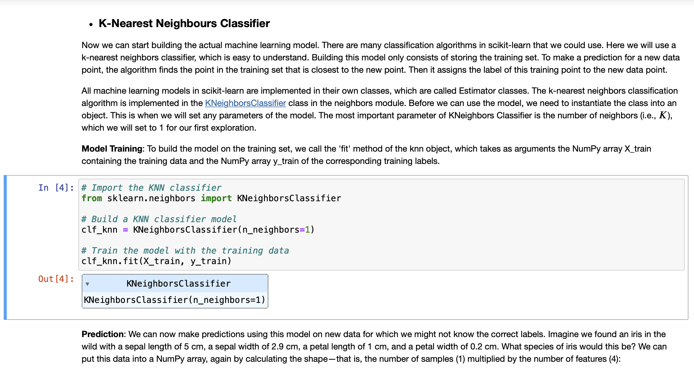
![In [5]: # Produce the features of a testing data instance X_new np.array([[5, 2.9, 1, 0.2]])](https://dsd5zvtm8ll6.cloudfront.net/si.experts.images/answers/2023/10/652025ea08939_674652025ea032f2.jpg)
![Task 4 Given the training data generated as follows: In [21]: X = np.array([[-1, -1], [-2, -1], [-3, -2], [1,](https://dsd5zvtm8ll6.cloudfront.net/si.experts.images/answers/2023/10/652025efada66_679652025efa931f.jpg)
![In [ ]: In [ ]: Comparasion on Iris data In [8]: # [Your code here Task 6 Compare the prediction accuaracy](https://dsd5zvtm8ll6.cloudfront.net/si.experts.images/answers/2023/10/652025f1e6b01_681652025f1e1f3c.jpg)
Transcribed Image Text:
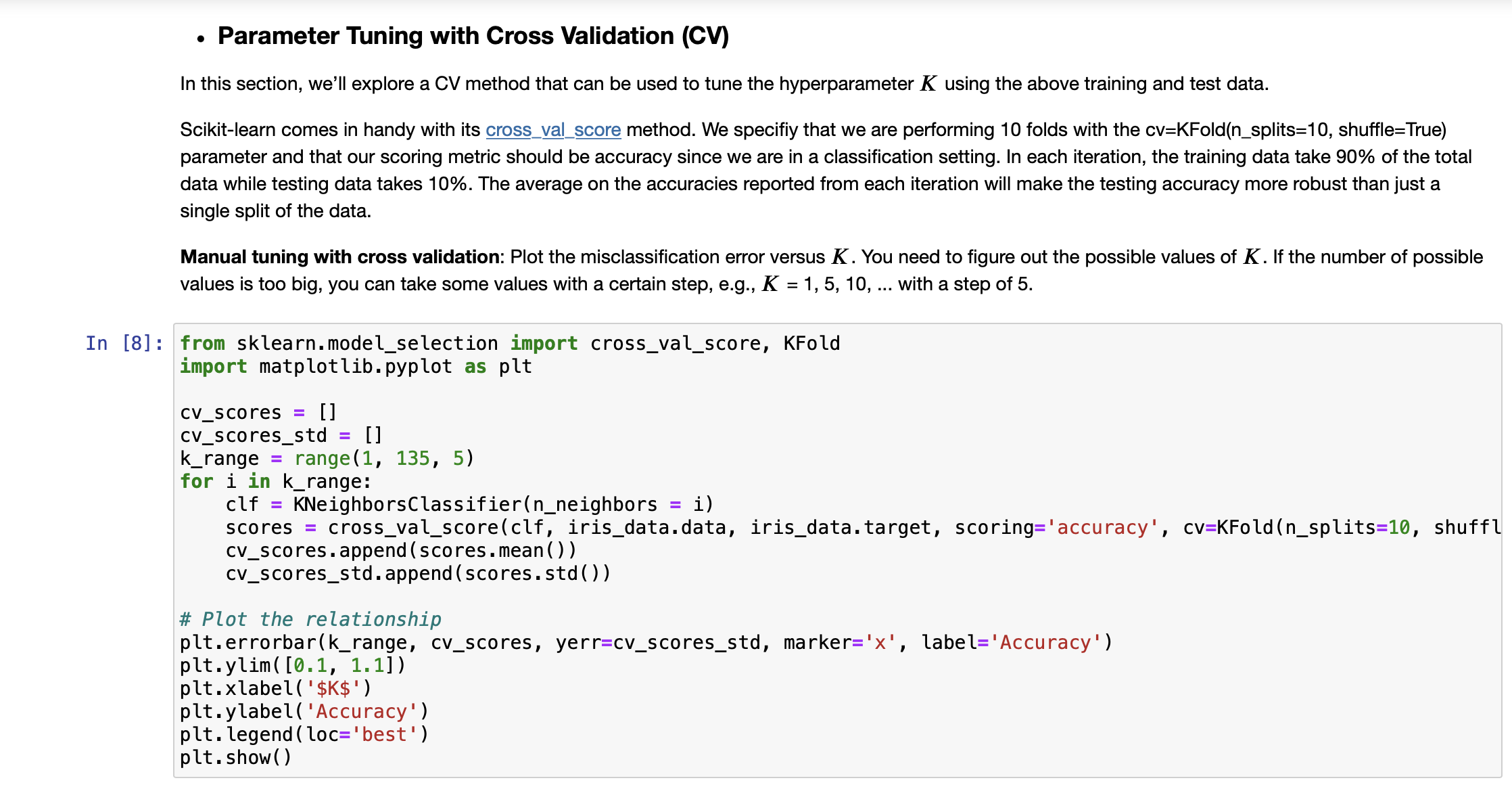
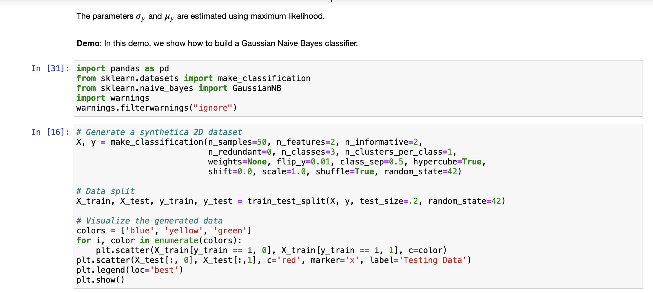
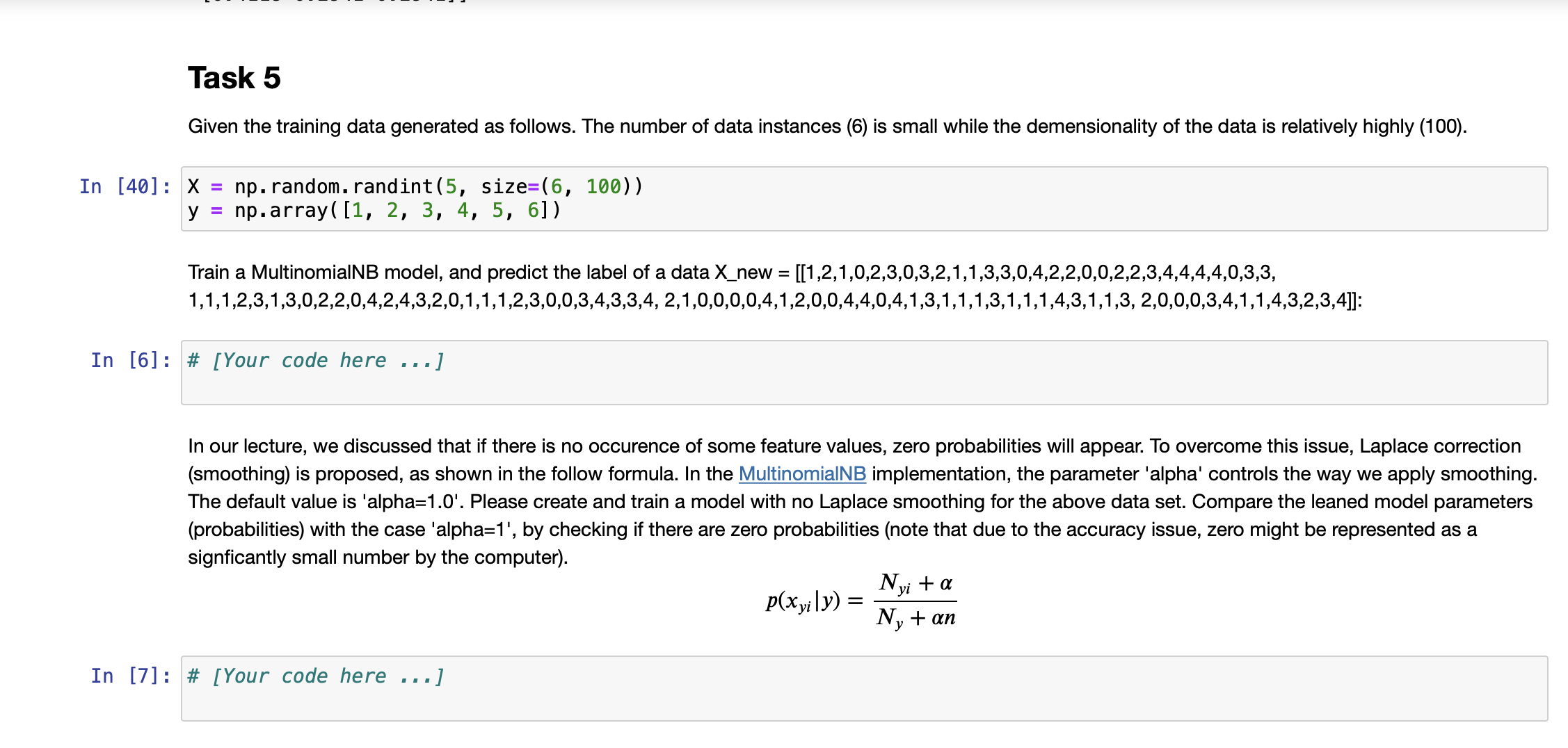
K-Nearest Neighbours Classifier Now we can start building the actual machine learning model. There are many classification algorithms in scikit-learn that we could use. Here we will use a k-nearest neighbors classifier, which is easy to understand. Building this model only consists of storing the training set. To make a prediction for a new data point, the algorithm finds the point in the training set that is closest to the new point. Then it assigns the label of this training point to the new data point. Out [4]: ● All machine learning models in scikit-learn are implemented in their own classes, which are called Estimator classes. The k-nearest neighbors classification algorithm is implemented in the KNeighbors Classifier class in the neighbors module. Before we can use the model, we need to instantiate the class into an object. This is when we will set any parameters of the model. The most important parameter of KNeighbors Classifier is the number of neighbors (i.e., K), which we will set to 1 for our first exploration. Model Training: To build the model on the training set, we call the 'fit' method of the knn object, which takes as arguments the NumPy array X_train containing the training data and the NumPy array y_train of the corresponding training labels. In [4] # Import the KNN classifier from sklearn.neighbors import KNeighborsClassifier # Build a KNN classifier model clf_knn KNeighbors Classifier(n_neighbors=1) # Train the model with the training data clf_knn.fit (X_train, y_train) KNeighbors Classifier KNeighbors Classifier (n_neighbors=1) Prediction: We can now make predictions using this model on new data for which we might not know the correct labels. Imagine we found an iris in the wild with a sepal length of 5 cm, a sepal width of 2.9 cm, a petal length of 1 cm, and a petal width of 0.2 cm. What species of iris would this be? We can put this data into a NumPy array, again by calculating the shape-that is, the number of samples (1) multiplied by the number of features (4): In [5]: # Produce the features of a testing data instance X_new np.array([[5, 2.9, 1, 0.2]]) print("X_new.shape: {}".format(X_new.shape)) # Predict the result label of X_new: y_new_pred = clf_knn.predict (X_new) print("The predicted class is: \n", y_new_pred) X_new.shape: (1, 4) The predicted class is: [0] Our model predicts that this new iris belongs to the class 0, meaning its species is setosa. But how do we know whether we can trust our model? We don't know the correct species of this sample, which is the whole point of building the model! Evaluating Model: This is where the test set that we created earlier comes in. This data was not used to build the model, but we do know what the correct species is for each iris in the test set. So, we can use the trained model to predict these data instances and calculate the accuracy to evaluate how good the model is. Task 1 Write code to calculate the accuracy score In [1] # [Your code here ...] Parameter Tuning with Cross Validation (CV) In this section, we'll explore a CV method that can be used to tune the hyperparameter K using the above training and test data. Scikit-learn comes in handy with its cross_val_score method. We specifiy that we are performing 10 folds with the cv=KFold(n_splits=10, shuffle=True) parameter and that our scoring metric should be accuracy since we are in a classification setting. In each iteration, the training data take 90% of the total data while testing data takes 10%. The average on the accuracies reported from each iteration will make the testing accuracy more robust than just a single split of the data. Manual tuning with cross validation: Plot the misclassification error versus K. You need to figure out the possible values of K. If the number of possible values is too big, you can take some values with a certain step, e.g., K = 1, 5, 10, ... with a step of 5. In [8]: from sklearn.model_ selection import cross_val_score, KFold import matplotlib.pyplot as plt cv_scores = [] cv_scores_std = [] k_range= range(1, 135, 5) for i in k_range: clf KNeighbors Classifier(n_neighbors scores = cross_val_score(clf, iris_data.data, iris_data.target, scoring='accuracy', cv=KFold (n_splits=10, shuffl cv_scores.append(scores.mean()) cv_scores_std.append(scores.std()) = i) #Plot the relationship plt.errorbar(k_range, cv_scores, yerr=cv_scores_std, marker='x', label='Accuracy') plt. ylim( [0.1, 1.1]) plt.xlabel('$K$') plt.ylabel('Accuracy') plt. legend (loc='best') plt.show() It can be seen that the accuracy first goes up when K increases. It peeks around 15. Then, it keeps going down. Particularly, the performance (measured by the score mean) and its robustness/stableness (measured by the score std) drop substantially around K=85. One possible reason is that when K is bigger than 85, the model suffers from the underfitting issue severely. Automated Parameter Tuning: Use the GridSearch CV method to accomplish automatic model selection. Task 2 Check against the figure plotted above to see if the selected hyperparameter K can lead to the highest misclassification accuracy. In [2] # [Your code here ...] Task 3 It can be seen that GridSearchCV can help us to the automated hyperparameter tuning. Actually, it also store the intermediate results during the search process. The attribute 'cv_results_' of GridSearchCV contains much such informaiton. For example, this attribute contains the 'mean_test_score' and 'std_test_score' for the cross validation. Make use of this information to produce a plot similar to what we did in the manual way. Please check if the two plots comply with each other. In [3]: # [Your code here ..] 2. Naive Bayes Classifier Naive Bayes methods are a set of supervised learning algorithms based on applying Bayes' theorem with the "naive" assumption of conditional independence between every pair of features given the value of the class variable. Bayes'theorem states the following relationship, given class variable y and dependent feature vector x₁ through xn, P(y | x₁, Using the naive conditional independence assumption, we have ,xn) P(y)P(x₁, . xn | y) P(x₁,...,xn) n P(y | x₁, ..., X₁) ∞ P(y)¶¶P(xz | y) xn) i=1 n ŷ = arg max P(y) | P(x₁ | y), y i=1 Then, we can use Maximum A Posteriori (MAP) estimation to estimate P(y) and P(x; | y); the former is then the relative frequency of class y in the training set. References: H. Zhang (2004). The optimality of Naive Bayes. Proc. FLAIRS. P(x¡ | y) = = Gaussian Naive Bayes GaussianNB implements the Gaussian Naive Bayes algorithm for classification on the data sets where features are continuous. The likelihood of the features is assumed to be Gaussian: 1 2πσ, P ( - (*₁ = 4₂)²2) (Xi 203 exp The parameters oy and μy are estimated using maximum likelihood. Demo: In this demo, we show how to build a Gaussian Naive Bayes classifier. In [31] import pandas as pd from sklearn.datasets import make_classification from sklearn.naive_bayes import GaussianNB import warnings warnings.filterwarnings("ignore") In [16]: # Generate a synthetica 2D dataset X, y = make_classification(n_samples=50, n_features=2, n_informative=2, n_redundant=0, n_classes=3, n_clusters_per_class=1, weights=None, flip_y=0.01, class_sep=0.5, hypercube=True, shift=0.0, scale=1.0, shuffle=True, random_state=42) # Data split X_train, X_test, y_train, y_test = train_test_split(X, y, test_size=.2, random_state=42) # Visualize the generated data colors = ['blue', 'yellow', 'green'] for i, color in enumerate (colors): plt.scatter (X_train[y_train i, 0], X_train [y_train i, 11, c-color) plt.scatter (X_test[:, 0], X_test[:,1], c='red', marker='x', label='Testing Data') plt. legend (loc='best') plt.show() == Task 4 Given the training data generated as follows: In [21]: X = np.array([[-1, −1], [-2, -1], [-3, -2], [1, 1], [2, 1], [3, 2]]) np.array([1, 1, 1, 2, 2, 2]) y = # Firstly, let's do the parameter estimation manually without using the model |X_0_C_1=X [y==1] [:,0] |X_1_C_1=X [y==1] [:,1] X_0_C_2=X [y==2][:,0] X_1_C_2=X [y==2][:,1] manual_means = np.array([[X_0_C_1.mean(), X_1_C_1.mean()], [X_0_C_2.mean(), X_1_C_2.mean()]]) np.set_printoptions(precision=4) print('Means estaimated manually: \n', manual_means) manual_vars = np.array([[X_0_C_1.var(), X_1_C_1.var()], [X_0_C_2.var(), X_1_C_2.var()]]) print('Variances estaimated manually: \n', manual_vars) Means estaimated manually: [[-2. -1.3333] [ 2. 1.3333]] Variances estaimated manually: [[0.6667 0.2222] [0.6667 0.2222]] Train a GaussianNB model and print out the learned model parameters (parameters of probability distributions). And check if the learned parameters comply with the manually estimated ones as shown above. Predict the label of a data [-0.8,-1]. In [4] # [Your code here ...] Task 5 Given the training data generated as follows. The number of data instances (6) is small while the demensionality of the data is relatively highly (100). In [40]: X = np. random.randint (5, size=(6, 100)) y np.array([1, 2, 3, 4, 5, 6]) Train a MultinomialNB model, and predict the label of a data X_new = [[1,2,1,0,2,3,0,3,2,1,1,3,3,0,4,2,2,0,0,2,2,3,4,4,4,4,0,3,3, 1,1,1,2,3,1,3,0,2,2,0,4,2,4,3,2,0,1,1,1,2,3,0,0,3,4,3,3,4, 2,1,0,0,0,0,4,1,2,0,0,4,4,0,4,1,3,1,1,1,3,1,1,1,4,3,1,1,3, 2,0,0,0,3,4,1,1,4,3,2,3,4]]: In [6] # [Your code here ...] In our lecture, we discussed that if there is no occurence of some feature values, zero probabilities will appear. To overcome this issue, Laplace correction (smoothing) is proposed, as shown in the follow formula. In the MultinomialNB implementation, the parameter 'alpha' controls the way we apply smoothing. The default value is 'alpha=1.0'. Please create and train a model with no Laplace smoothing for the above data set. Compare the leaned model parameters (probabilities) with the case 'alpha=1', by checking if there are zero probabilities (note that due to the accuracy issue, zero might be represented as a signficantly small number by the computer). In [7] # [Your code here ...] p(xyily) = Nyi + a Ny + an In [ ]: ● In [ ]: Comparasion on Iris data In [8] # [Your code here Task 6 Compare the prediction accuaracy between KNN clasifier (use the optimal K you've identied) and Gaussian Naive Bayes. Use 10-cross validation to report the accuracy mean and standard deviation (Note this is to ensure the comparison is based on robust performace). Which classifidation mdoel is more accurate on Iris data set? Use t-test to show if the difference is statistically significant. .] K-Nearest Neighbours Classifier Now we can start building the actual machine learning model. There are many classification algorithms in scikit-learn that we could use. Here we will use a k-nearest neighbors classifier, which is easy to understand. Building this model only consists of storing the training set. To make a prediction for a new data point, the algorithm finds the point in the training set that is closest to the new point. Then it assigns the label of this training point to the new data point. Out [4]: ● All machine learning models in scikit-learn are implemented in their own classes, which are called Estimator classes. The k-nearest neighbors classification algorithm is implemented in the KNeighbors Classifier class in the neighbors module. Before we can use the model, we need to instantiate the class into an object. This is when we will set any parameters of the model. The most important parameter of KNeighbors Classifier is the number of neighbors (i.e., K), which we will set to 1 for our first exploration. Model Training: To build the model on the training set, we call the 'fit' method of the knn object, which takes as arguments the NumPy array X_train containing the training data and the NumPy array y_train of the corresponding training labels. In [4] # Import the KNN classifier from sklearn.neighbors import KNeighborsClassifier # Build a KNN classifier model clf_knn KNeighbors Classifier(n_neighbors=1) # Train the model with the training data clf_knn.fit (X_train, y_train) KNeighbors Classifier KNeighbors Classifier (n_neighbors=1) Prediction: We can now make predictions using this model on new data for which we might not know the correct labels. Imagine we found an iris in the wild with a sepal length of 5 cm, a sepal width of 2.9 cm, a petal length of 1 cm, and a petal width of 0.2 cm. What species of iris would this be? We can put this data into a NumPy array, again by calculating the shape-that is, the number of samples (1) multiplied by the number of features (4): In [5]: # Produce the features of a testing data instance X_new np.array([[5, 2.9, 1, 0.2]]) print("X_new.shape: {}".format(X_new.shape)) # Predict the result label of X_new: y_new_pred = clf_knn.predict (X_new) print("The predicted class is: \n", y_new_pred) X_new.shape: (1, 4) The predicted class is: [0] Our model predicts that this new iris belongs to the class 0, meaning its species is setosa. But how do we know whether we can trust our model? We don't know the correct species of this sample, which is the whole point of building the model! Evaluating Model: This is where the test set that we created earlier comes in. This data was not used to build the model, but we do know what the correct species is for each iris in the test set. So, we can use the trained model to predict these data instances and calculate the accuracy to evaluate how good the model is. Task 1 Write code to calculate the accuracy score In [1] # [Your code here ...] Parameter Tuning with Cross Validation (CV) In this section, we'll explore a CV method that can be used to tune the hyperparameter K using the above training and test data. Scikit-learn comes in handy with its cross_val_score method. We specifiy that we are performing 10 folds with the cv=KFold(n_splits=10, shuffle=True) parameter and that our scoring metric should be accuracy since we are in a classification setting. In each iteration, the training data take 90% of the total data while testing data takes 10%. The average on the accuracies reported from each iteration will make the testing accuracy more robust than just a single split of the data. Manual tuning with cross validation: Plot the misclassification error versus K. You need to figure out the possible values of K. If the number of possible values is too big, you can take some values with a certain step, e.g., K = 1, 5, 10, ... with a step of 5. In [8]: from sklearn.model_ selection import cross_val_score, KFold import matplotlib.pyplot as plt cv_scores = [] cv_scores_std = [] k_range= range(1, 135, 5) for i in k_range: clf KNeighbors Classifier(n_neighbors scores = cross_val_score(clf, iris_data.data, iris_data.target, scoring='accuracy', cv=KFold (n_splits=10, shuffl cv_scores.append(scores.mean()) cv_scores_std.append(scores.std()) = i) #Plot the relationship plt.errorbar(k_range, cv_scores, yerr=cv_scores_std, marker='x', label='Accuracy') plt. ylim( [0.1, 1.1]) plt.xlabel('$K$') plt.ylabel('Accuracy') plt. legend (loc='best') plt.show() It can be seen that the accuracy first goes up when K increases. It peeks around 15. Then, it keeps going down. Particularly, the performance (measured by the score mean) and its robustness/stableness (measured by the score std) drop substantially around K=85. One possible reason is that when K is bigger than 85, the model suffers from the underfitting issue severely. Automated Parameter Tuning: Use the GridSearch CV method to accomplish automatic model selection. Task 2 Check against the figure plotted above to see if the selected hyperparameter K can lead to the highest misclassification accuracy. In [2] # [Your code here ...] Task 3 It can be seen that GridSearchCV can help us to the automated hyperparameter tuning. Actually, it also store the intermediate results during the search process. The attribute 'cv_results_' of GridSearchCV contains much such informaiton. For example, this attribute contains the 'mean_test_score' and 'std_test_score' for the cross validation. Make use of this information to produce a plot similar to what we did in the manual way. Please check if the two plots comply with each other. In [3]: # [Your code here ..] 2. Naive Bayes Classifier Naive Bayes methods are a set of supervised learning algorithms based on applying Bayes' theorem with the "naive" assumption of conditional independence between every pair of features given the value of the class variable. Bayes'theorem states the following relationship, given class variable y and dependent feature vector x₁ through xn, P(y | x₁, Using the naive conditional independence assumption, we have ,xn) P(y)P(x₁, . xn | y) P(x₁,...,xn) n P(y | x₁, ..., X₁) ∞ P(y)¶¶P(xz | y) xn) i=1 n ŷ = arg max P(y) | P(x₁ | y), y i=1 Then, we can use Maximum A Posteriori (MAP) estimation to estimate P(y) and P(x; | y); the former is then the relative frequency of class y in the training set. References: H. Zhang (2004). The optimality of Naive Bayes. Proc. FLAIRS. P(x¡ | y) = = Gaussian Naive Bayes GaussianNB implements the Gaussian Naive Bayes algorithm for classification on the data sets where features are continuous. The likelihood of the features is assumed to be Gaussian: 1 2πσ, P ( - (*₁ = 4₂)²2) (Xi 203 exp The parameters oy and μy are estimated using maximum likelihood. Demo: In this demo, we show how to build a Gaussian Naive Bayes classifier. In [31] import pandas as pd from sklearn.datasets import make_classification from sklearn.naive_bayes import GaussianNB import warnings warnings.filterwarnings("ignore") In [16]: # Generate a synthetica 2D dataset X, y = make_classification(n_samples=50, n_features=2, n_informative=2, n_redundant=0, n_classes=3, n_clusters_per_class=1, weights=None, flip_y=0.01, class_sep=0.5, hypercube=True, shift=0.0, scale=1.0, shuffle=True, random_state=42) # Data split X_train, X_test, y_train, y_test = train_test_split(X, y, test_size=.2, random_state=42) # Visualize the generated data colors = ['blue', 'yellow', 'green'] for i, color in enumerate (colors): plt.scatter (X_train[y_train i, 0], X_train [y_train i, 11, c-color) plt.scatter (X_test[:, 0], X_test[:,1], c='red', marker='x', label='Testing Data') plt. legend (loc='best') plt.show() == Task 4 Given the training data generated as follows: In [21]: X = np.array([[-1, −1], [-2, -1], [-3, -2], [1, 1], [2, 1], [3, 2]]) np.array([1, 1, 1, 2, 2, 2]) y = # Firstly, let's do the parameter estimation manually without using the model |X_0_C_1=X [y==1] [:,0] |X_1_C_1=X [y==1] [:,1] X_0_C_2=X [y==2][:,0] X_1_C_2=X [y==2][:,1] manual_means = np.array([[X_0_C_1.mean(), X_1_C_1.mean()], [X_0_C_2.mean(), X_1_C_2.mean()]]) np.set_printoptions(precision=4) print('Means estaimated manually: \n', manual_means) manual_vars = np.array([[X_0_C_1.var(), X_1_C_1.var()], [X_0_C_2.var(), X_1_C_2.var()]]) print('Variances estaimated manually: \n', manual_vars) Means estaimated manually: [[-2. -1.3333] [ 2. 1.3333]] Variances estaimated manually: [[0.6667 0.2222] [0.6667 0.2222]] Train a GaussianNB model and print out the learned model parameters (parameters of probability distributions). And check if the learned parameters comply with the manually estimated ones as shown above. Predict the label of a data [-0.8,-1]. In [4] # [Your code here ...] Task 5 Given the training data generated as follows. The number of data instances (6) is small while the demensionality of the data is relatively highly (100). In [40]: X = np. random.randint (5, size=(6, 100)) y np.array([1, 2, 3, 4, 5, 6]) Train a MultinomialNB model, and predict the label of a data X_new = [[1,2,1,0,2,3,0,3,2,1,1,3,3,0,4,2,2,0,0,2,2,3,4,4,4,4,0,3,3, 1,1,1,2,3,1,3,0,2,2,0,4,2,4,3,2,0,1,1,1,2,3,0,0,3,4,3,3,4, 2,1,0,0,0,0,4,1,2,0,0,4,4,0,4,1,3,1,1,1,3,1,1,1,4,3,1,1,3, 2,0,0,0,3,4,1,1,4,3,2,3,4]]: In [6] # [Your code here ...] In our lecture, we discussed that if there is no occurence of some feature values, zero probabilities will appear. To overcome this issue, Laplace correction (smoothing) is proposed, as shown in the follow formula. In the MultinomialNB implementation, the parameter 'alpha' controls the way we apply smoothing. The default value is 'alpha=1.0'. Please create and train a model with no Laplace smoothing for the above data set. Compare the leaned model parameters (probabilities) with the case 'alpha=1', by checking if there are zero probabilities (note that due to the accuracy issue, zero might be represented as a signficantly small number by the computer). In [7] # [Your code here ...] p(xyily) = Nyi + a Ny + an In [ ]: ● In [ ]: Comparasion on Iris data In [8] # [Your code here Task 6 Compare the prediction accuaracy between KNN clasifier (use the optimal K you've identied) and Gaussian Naive Bayes. Use 10-cross validation to report the accuracy mean and standard deviation (Note this is to ensure the comparison is based on robust performace). Which classifidation mdoel is more accurate on Iris data set? Use t-test to show if the difference is statistically significant. .]
Expert Answer:
Answer rating: 100% (QA)
It seems that you have a series of tasks related to machine learning classification models specifically the kNearest Neighbors kNN classifier and the Naive Bayes classifier These tasks involve impleme... View the full answer

Related Book For 

Financial Accounting and Reporting a Global Perspective
ISBN: 978-1408076866
4th edition
Authors: Michel Lebas, Herve Stolowy, Yuan Ding
Posted Date:
Students also viewed these programming questions
-
The ABC team estimated that for the three pilot-test bank branches, the retail and business customer lines experienced the annual activity levels(inthousands) as shown in Exhibit C. For example,...
-
Compare and contrast cognitive psychology and behaviorism? what are some cognitive psychology and behaviorism potential uses in therapy? with examples. how might you use cognitive psychology (or...
-
K-Nearest Neighbours Classifier Now we can start building the actual machine learning model. There are many classification algorithms in scikit-learn that we could use. Here we will use a k-nearest...
-
Use the Ratio Test to determine if each series converges absolutely or diverges. 8 n=1 nt (-4)"
-
In general, are chi-square distributions symmetric or skewed? If skewed, are they skewed right or left?
-
Skousen Exploration Corporation was formed on January 1, 20X3. The company was formed by Cliff and Chris Skousen with the goal of conducting geophysical support services related to natural gas...
-
On June 1, 2020, Athletes Inc. sold 400 shares of Spartan stock for \(\$ 33\) per share and 100 shares of Wildcat stock for \(\$ 55\) per share. Athletes Inc. purchased 400 shares of Gopher common...
-
Austin Enterprises makes and sells three types of dress shirts. Management is trying to determine the most profitable mix. Sales prices, demand, and use of manufacturing inputs follow: The company...
-
Transoceanic Airlines is examining a resort motel chain to addto its operations. Before the acquisition, the normal expectedoutcomes for the firm were as follows: Outcomes($ millions)Probab 2 answers
-
Review the calculations for The Diamond Ridge Golf Course example discussed in the chapter. 1. Based on these calculations, is there any good-will value? If so, how much? 2. How did you make this...
-
Suppose the following are measurements of the temperature T (in degrees Celsius) and insects sizes S (in millimiters) T 10 20 30 5 0.2 0.1 0 S 20 0.1 0.2 0.1 80 0 0.1 0.2 (i) Find the correlation...
-
Explain at least two of the following:Indirect costs, direct costs, allocation base, pool, G&A, fringe benefits, intermediate pools, and under/over applied overhead.Discuss how the two you selected...
-
Mr. Burns has asked you to do the following as part of your analysis of the capital investment project. 3. Identify possible flaws in the numbers or assumptions used in the analysis, and identify the...
-
Explain how the Spanning Tree Protocol works and its impact on physical loops between bridges and switches. What kind of problems would logical loops pose for packets delivery? Also, how do you think...
-
Villa Company's standard cost system contains the following overhead costs, computed based on a monthly normal volume of 25,000 units or 50,000 direct labor hours: Variable factory overhead P12 per...
-
How do costs flow through a process costing system? What are equivalent units of production, and how are they calculated? How is a production cost report prepared for the first department? How is a...
-
The balance sheet contains a section for the cash related to invest in both fixed assets and securities used as alternative to cash holding. (T/F) Depreciation would be listed on the asset section of...
-
Pearson Education, a publisher of college textbooks, would like to know if students prefer traditional textbooks or digital textbooks. A random sample of students was asked their preference and the...
-
Holmen (formerly MoDo), is a Swedish group manufacturing and selling newsprint and magazine paper as well as paperboard. Its financial statements are prepared in accordance with IFRS. The 2010 and...
-
Wipro Limited, together with its subsidiaries and equity accounted investees (collectively, Wipro) is a leading India-based provider of IT Services, including Business Process Outsourcing (BPO)...
-
Nokia (Finland) is still among the leaders in the telecommunication industry, with emphasis on cellular phones and other wireless solutions. The consolidated financial statements are prepared in...
-
The question is the same as in problem 5 , but now the simple implicit scheme (6.34) is used. Consider two situations. a) The expected error must be less than \(\sim 10^{-4}\) for the entire...
-
Compare the schemes introduced for the linear convection equation. a) Simple explicit schemes (7.6), (7.7), and (7.8) b) Simple implicit scheme (7.19) c) Leapfrog scheme (7.21) d) Lax-Wendroff scheme...
-
Repeat Problem 7.1 for the following schemes applied to the one-dimensional heat equation. a) Simple explicit scheme \((7.28)\) b) Simple implicit scheme \((7.32)\) c) Crank-Nicolson scheme (7.34)...

Study smarter with the SolutionInn App