K-Nearest Neighbours Classifier Now we can start building the actual machine learning model. There are many...

Transcribed Image Text:

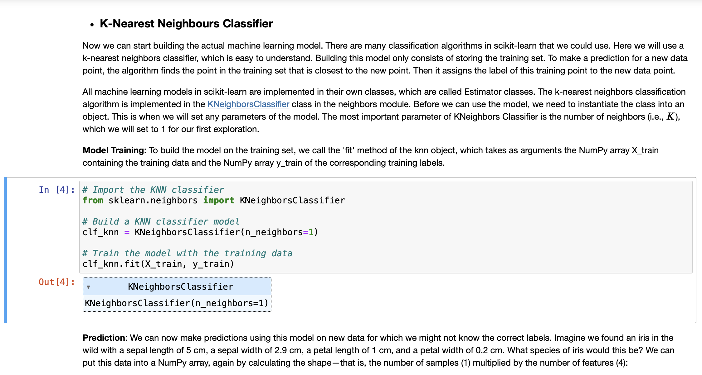
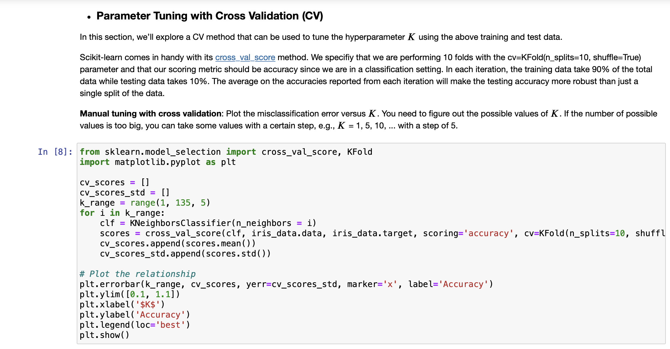
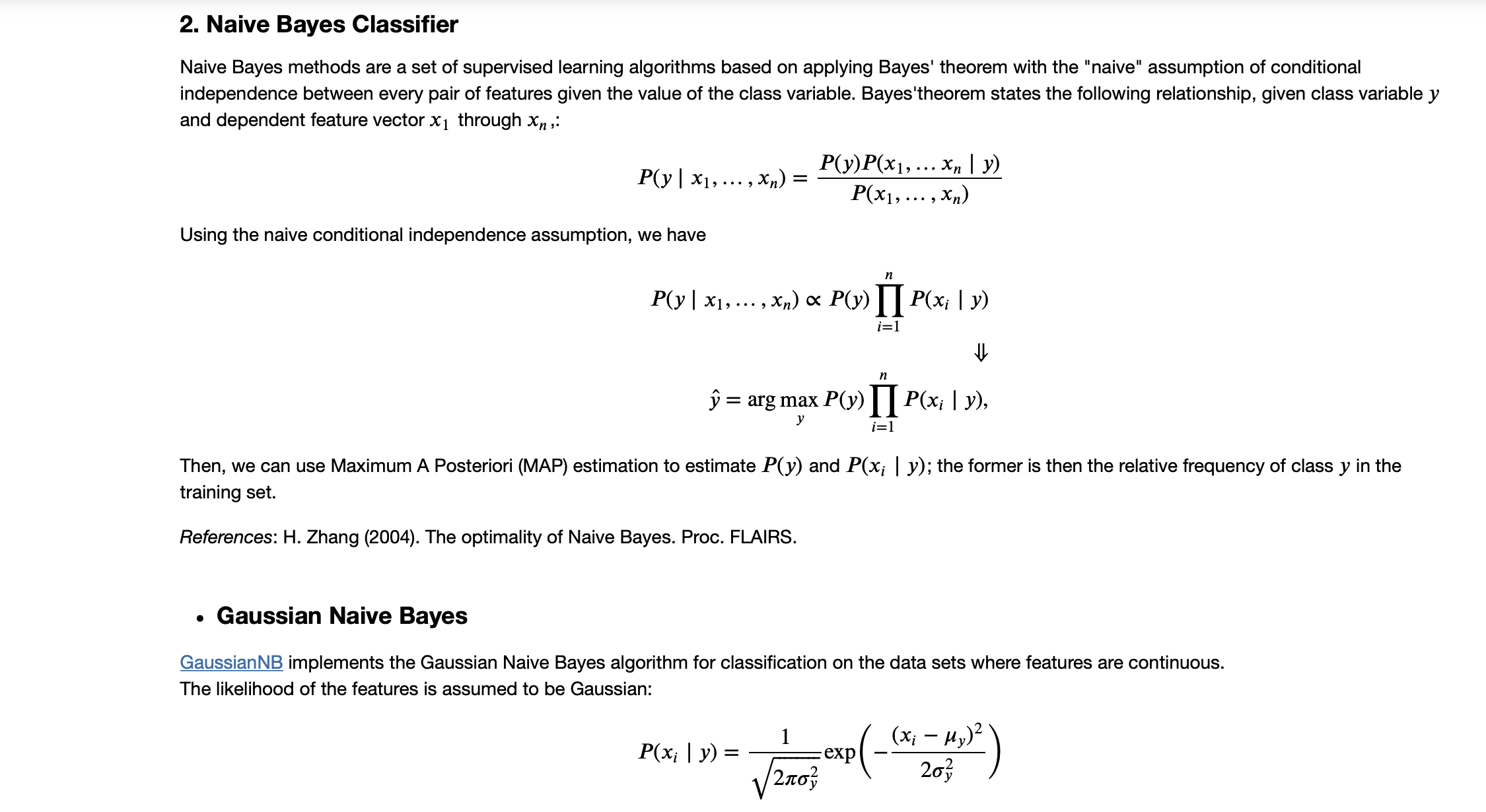
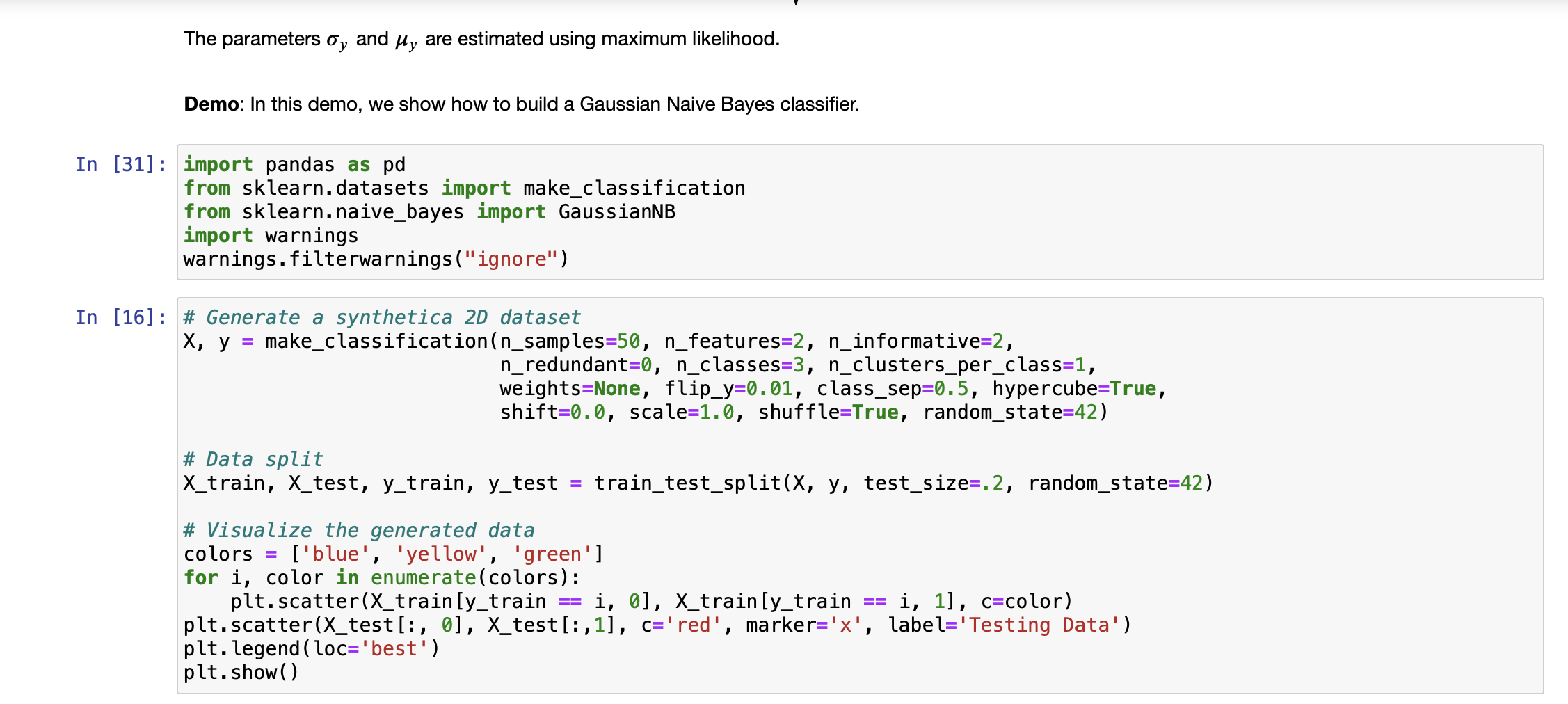
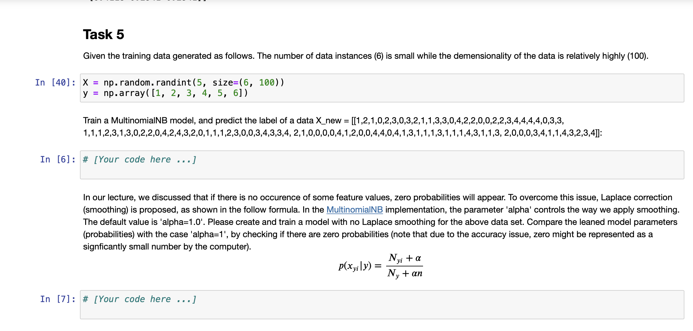
K-Nearest Neighbours Classifier Now we can start building the actual machine learning model. There are many classification algorithms in scikit-learn that we could use. Here we will use a k-nearest neighbors classifier, which is easy to understand. Building this model only consists of storing the training set. To make a prediction for a new data point, the algorithm finds the point in the training set that is closest to the new point. Then it assigns the label of this training point to the new data point. Out [4]: ● All machine learning models in scikit-learn are implemented in their own classes, which are called Estimator classes. The k-nearest neighbors classification algorithm is implemented in the KNeighbors Classifier class in the neighbors module. Before we can use the model, we need to instantiate the class into an object. This is when we will set any parameters of the model. The most important parameter of KNeighbors Classifier is the number of neighbors (i.e., K), which we will set to 1 for our first exploration. Model Training: To build the model on the training set, we call the 'fit' method of the knn object, which takes as arguments the NumPy array X_train containing the training data and the NumPy array y_train of the corresponding training labels. In [4] # Import the KNN classifier from sklearn.neighbors import KNeighborsClassifier # Build a KNN classifier model clf_knn KNeighbors Classifier(n_neighbors=1) # Train the model with the training data clf_knn.fit (X_train, y_train) KNeighbors Classifier KNeighbors Classifier (n_neighbors=1) Prediction: We can now make predictions using this model on new data for which we might not know the correct labels. Imagine we found an iris in the wild with a sepal length of 5 cm, a sepal width of 2.9 cm, a petal length of 1 cm, and a petal width of 0.2 cm. What species of iris would this be? We can put this data into a NumPy array, again by calculating the shape-that is, the number of samples (1) multiplied by the number of features (4): In [5]: # Produce the features of a testing data instance X_new np.array([[5, 2.9, 1, 0.2]]) print("X_new.shape: {}".format(X_new.shape)) #Predict the result label of X_new: y_new_pred = clf_knn.predict (X_new) print("The predicted class is: \n", y_new_pred) X_new.shape: (1, 4) The predicted class is: [0] Our model predicts that this new iris belongs to the class 0, meaning its species is setosa. But how do we know whether we can trust our model? We don't know the correct species of this sample, which is the whole point of building the model! Evaluating Model: This is where the test set that we created earlier comes in. This data was not used to build the model, but we do know what the correct species is for each iris in the test set. So, we can use the trained model to predict these data instances and calculate the accuracy to evaluate how good the model is. Task 1 Write code to calculate the accuracy score In [1] # [Your code here ...] Parameter Tuning with Cross Validation (CV) In this section, we'll explore a CV method that can be used to tune the hyperparameter K using the above training and test data. Scikit-learn comes in handy with its cross_val_score method. We specifiy that we are performing 10 folds with the cv=KFold(n_splits=10, shuffle=True) parameter and that our scoring metric should be accuracy since we are in a classification setting. In each iteration, the training data take 90% of the total data while testing data takes 10%. The average on the accuracies reported from each iteration will make the testing accuracy more robust than just a single split of the data. Manual tuning with cross validation: Plot the misclassification error versus K. You need to figure out the possible values of K. If the number of possible values is too big, you can take some values with a certain step, e.g., K = 1, 5, 10, ... with a step of 5. In [8]: from sklearn.model_selection import cross_val_score, KFold import matplotlib.pyplot as plt cv_scores = [] cv_scores_std = [] k_range= range(1, 135, 5) for i in k_range: clf KNeighbors Classifier(n_neighbors scores = cross_val_score(clf, iris_data.data, iris_data.target, scoring='accuracy', cv=KFold (n_splits=10, shuffl cv_scores.append(scores.mean()) cv_scores_std.append(scores.std()) = i) #Plot the relationship plt.errorbar(k_range, cv_scores, yerr=cv_scores_std, marker='x', label='Accuracy') plt.ylim( [0.1, 1.1]) plt.xlabel('$K$') plt.ylabel('Accuracy') plt. legend (loc='best') plt.show() It can be seen that the accuracy first goes up when K increases. It peeks around 15. Then, it keeps going down. Particularly, the performance (measured by the score mean) and its robustness/stableness (measured by the score std) drop substantially around K=85. One possible reason is that when K is bigger than 85, the model suffers from the underfitting issue severely. Automated Parameter Tuning: Use the GridSearchCV method to accomplish automatic model selection. Task 2 Check against the figure plotted above to see if the selected hyperparameter K can lead to the highest misclassification accuracy. In [2] # [Your code here ...] Task 3 It can be seen that GridSearchCV can help us to the automated hyperparameter tuning. Actually, it also store the intermediate results during the search process. The attribute 'cv_results_' of GridSearchCV contains much such informaiton. For example, this attribute contains the 'mean_test_score' and 'std_test_score' for the cross validation. Make use of this information to produce a plot similar to what we did in the manual way. Please check if the two plots comply with each other. In [3]: # [Your code here ..] 2. Naive Bayes Classifier Naive Bayes methods are a set of supervised learning algorithms based on applying Bayes' theorem with the "naive" assumption of conditional independence between every pair of features given the value of the class variable. Bayes'theorem states the following relationship, given class variable y and dependent feature vector x₁ through xn, P(y | x₁, Using the naive conditional independence assumption, we have ,xn) P(y)P(x₁, . xn | y) P(x₁,...,xn) n P(y | x₁, ..., Xn) × P(y)¶¶P(xi | y) ∞ i=1 n ŷ = arg max P(y) | P(x₁ | y), y i=1 Then, we can use Maximum A Posteriori (MAP) estimation to estimate P(y) and P(x; | y); the former is then the relative frequency of class y in the training set. References: H. Zhang (2004). The optimality of Naive Bayes. Proc. FLAIRS. P(x¡ | y) = = Gaussian Naive Bayes Gaussian NB implements the Gaussian Naive Bayes algorithm for classification on the data sets where features are continuous. The likelihood of the features is assumed to be Gaussian: 1 2πσ, P ( - (* ₁ = 1,)²2) 203 exp The parameters oy and μy are estimated using maximum likelihood. Demo: In this demo, we show how to build a Gaussian Naive Bayes classifier. In [31] import pandas as pd from sklearn.datasets import make_classification from sklearn.naive_bayes import GaussianNB import warnings warnings.filterwarnings("ignore") In [16]: # Generate a synthetica 2D dataset X, y = make_classification(n_samples=50, n_features=2, n_informative=2, n_redundant=0, n_classes=3, n_clusters_per_class=1, weights=None, flip_y=0.01, class_sep=0.5, hypercube=True, shift=0.0, scale=1.0, shuffle=True, random_state=42) # Data split X_train, X_test, y_train, y_test = train_test_split(X, y, test_size=.2, random_state=42) # Visualize the generated data colors = ['blue', 'yellow', 'green'] for i, color in enumerate (colors): plt.scatter (X_train[y_train i, 0], X_train [y_train i, 1], c-color) plt.scatter (X_test[:, 0], X_test[:,1], c='red', marker='x', label='Testing Data') plt. legend (loc='best') plt.show() == Task 4 Given the training data generated as follows: In [21]: X = np.array([[-1, -1], [-2, -1], [-3, -2], [1, 1], [2, 1], [3, 2]]) np.array([1, 1, 1, 2, 2, 2]) y = # Firstly, let's do the parameter estimation manually without using the model |X_0_C_1=X [y==1] [:,0] |X_1_C_1=X [y==1] [:,1] X_0_C_2=X [y==2][:,0] X_1_C_2=X [y==2][:,1] manual_means = np.array([[X_0_C_1.mean(), X_1_C_1.mean()], [X_0_C_2.mean(), X_1_C_2.mean()]]) np.set_printoptions(precision=4) print('Means estaimated manually: \n', manual_means) manual_vars = np.array([[X_0_C_1.var(), X_1_C_1.var()], [X_0_C_2.var(), X_1_C_2.var()]]) print('Variances estaimated manually: \n', manual_vars) Means estaimated manually: [[-2. -1.3333] [ 2. 1.3333]] Variances estaimated manually: [[0.6667 0.2222] [0.6667 0.2222]] Train a GaussianNB model and print out the learned model parameters (parameters of probability distributions). And check if the learned parameters comply with the manually estimated ones as shown above. Predict the label of a data [-0.8,-1]. In [4]: # [Your code here ...] Task 5 Given the training data generated as follows. The number of data instances (6) is small while the demensionality of the data is relatively highly (100). In [40]: X = np. random.randint (5, size=(6, 100)) y np.array([1, 2, 3, 4, 5, 6]) Train a MultinomialNB model, and predict the label of a data X_new = [[1,2,1,0,2,3,0,3,2,1,1,3,3,0,4,2,2,0,0,2,2,3,4,4,4,4,0,3,3, 1,1,1,2,3,1,3,0,2,2,0,4,2,4,3,2,0,1,1,1,2,3,0,0,3,4,3,3,4, 2, 1,0,0,0,0,4,1,2,0,0,4,4,0,4,1,3,1,1,1,3,1,1,1,4,3,1,1,3, 2,0,0,0,3,4,1,1,4,3,2,3,4]]: In [6]: # [Your code here ...] In our lecture, we discussed that if there is no occurence of some feature values, zero probabilities will appear. To overcome this issue, Laplace correction (smoothing) is proposed, as shown in the follow formula. In the MultinomialNB implementation, the parameter 'alpha' controls the way we apply smoothing. The default value is 'alpha=1.0'. Please create and train a model with no Laplace smoothing for the above data set. Compare the leaned model parameters (probabilities) with the case 'alpha=1', by checking if there are zero probabilities (note that due to the accuracy issue, zero might be represented as a signficantly small number by the computer). In [7]: # [Your code here ...] p(xyily) = Nyi + a Ny + an In [ ]: ● In [ ]: Comparasion on Iris data In [8]: # [Your code here Task 6 Compare the prediction accuaracy between KNN clasifier (use the optimal K you've identied) and Gaussian Naive Bayes. Use 10-cross validation to report the accuracy mean and standard deviation (Note this is to ensure the comparison is based on robust performace). Which classifidation mdoel is more accurate on Iris data set? Use t-test to show if the difference is statistically significant. .] K-Nearest Neighbours Classifier Now we can start building the actual machine learning model. There are many classification algorithms in scikit-learn that we could use. Here we will use a k-nearest neighbors classifier, which is easy to understand. Building this model only consists of storing the training set. To make a prediction for a new data point, the algorithm finds the point in the training set that is closest to the new point. Then it assigns the label of this training point to the new data point. Out [4]: ● All machine learning models in scikit-learn are implemented in their own classes, which are called Estimator classes. The k-nearest neighbors classification algorithm is implemented in the KNeighbors Classifier class in the neighbors module. Before we can use the model, we need to instantiate the class into an object. This is when we will set any parameters of the model. The most important parameter of KNeighbors Classifier is the number of neighbors (i.e., K), which we will set to 1 for our first exploration. Model Training: To build the model on the training set, we call the 'fit' method of the knn object, which takes as arguments the NumPy array X_train containing the training data and the NumPy array y_train of the corresponding training labels. In [4] # Import the KNN classifier from sklearn.neighbors import KNeighborsClassifier # Build a KNN classifier model clf_knn KNeighbors Classifier(n_neighbors=1) # Train the model with the training data clf_knn.fit (X_train, y_train) KNeighbors Classifier KNeighbors Classifier (n_neighbors=1) Prediction: We can now make predictions using this model on new data for which we might not know the correct labels. Imagine we found an iris in the wild with a sepal length of 5 cm, a sepal width of 2.9 cm, a petal length of 1 cm, and a petal width of 0.2 cm. What species of iris would this be? We can put this data into a NumPy array, again by calculating the shape-that is, the number of samples (1) multiplied by the number of features (4): In [5]: # Produce the features of a testing data instance X_new np.array([[5, 2.9, 1, 0.2]]) print("X_new.shape: {}".format(X_new.shape)) #Predict the result label of X_new: y_new_pred = clf_knn.predict (X_new) print("The predicted class is: \n", y_new_pred) X_new.shape: (1, 4) The predicted class is: [0] Our model predicts that this new iris belongs to the class 0, meaning its species is setosa. But how do we know whether we can trust our model? We don't know the correct species of this sample, which is the whole point of building the model! Evaluating Model: This is where the test set that we created earlier comes in. This data was not used to build the model, but we do know what the correct species is for each iris in the test set. So, we can use the trained model to predict these data instances and calculate the accuracy to evaluate how good the model is. Task 1 Write code to calculate the accuracy score In [1] # [Your code here ...] Parameter Tuning with Cross Validation (CV) In this section, we'll explore a CV method that can be used to tune the hyperparameter K using the above training and test data. Scikit-learn comes in handy with its cross_val_score method. We specifiy that we are performing 10 folds with the cv=KFold(n_splits=10, shuffle=True) parameter and that our scoring metric should be accuracy since we are in a classification setting. In each iteration, the training data take 90% of the total data while testing data takes 10%. The average on the accuracies reported from each iteration will make the testing accuracy more robust than just a single split of the data. Manual tuning with cross validation: Plot the misclassification error versus K. You need to figure out the possible values of K. If the number of possible values is too big, you can take some values with a certain step, e.g., K = 1, 5, 10, ... with a step of 5. In [8]: from sklearn.model_selection import cross_val_score, KFold import matplotlib.pyplot as plt cv_scores = [] cv_scores_std = [] k_range= range(1, 135, 5) for i in k_range: clf KNeighbors Classifier(n_neighbors scores = cross_val_score(clf, iris_data.data, iris_data.target, scoring='accuracy', cv=KFold (n_splits=10, shuffl cv_scores.append(scores.mean()) cv_scores_std.append(scores.std()) = i) #Plot the relationship plt.errorbar(k_range, cv_scores, yerr=cv_scores_std, marker='x', label='Accuracy') plt.ylim( [0.1, 1.1]) plt.xlabel('$K$') plt.ylabel('Accuracy') plt. legend (loc='best') plt.show() It can be seen that the accuracy first goes up when K increases. It peeks around 15. Then, it keeps going down. Particularly, the performance (measured by the score mean) and its robustness/stableness (measured by the score std) drop substantially around K=85. One possible reason is that when K is bigger than 85, the model suffers from the underfitting issue severely. Automated Parameter Tuning: Use the GridSearchCV method to accomplish automatic model selection. Task 2 Check against the figure plotted above to see if the selected hyperparameter K can lead to the highest misclassification accuracy. In [2] # [Your code here ...] Task 3 It can be seen that GridSearchCV can help us to the automated hyperparameter tuning. Actually, it also store the intermediate results during the search process. The attribute 'cv_results_' of GridSearchCV contains much such informaiton. For example, this attribute contains the 'mean_test_score' and 'std_test_score' for the cross validation. Make use of this information to produce a plot similar to what we did in the manual way. Please check if the two plots comply with each other. In [3]: # [Your code here ..] 2. Naive Bayes Classifier Naive Bayes methods are a set of supervised learning algorithms based on applying Bayes' theorem with the "naive" assumption of conditional independence between every pair of features given the value of the class variable. Bayes'theorem states the following relationship, given class variable y and dependent feature vector x₁ through xn, P(y | x₁, Using the naive conditional independence assumption, we have ,xn) P(y)P(x₁, . xn | y) P(x₁,...,xn) n P(y | x₁, ..., Xn) × P(y)¶¶P(xi | y) ∞ i=1 n ŷ = arg max P(y) | P(x₁ | y), y i=1 Then, we can use Maximum A Posteriori (MAP) estimation to estimate P(y) and P(x; | y); the former is then the relative frequency of class y in the training set. References: H. Zhang (2004). The optimality of Naive Bayes. Proc. FLAIRS. P(x¡ | y) = = Gaussian Naive Bayes Gaussian NB implements the Gaussian Naive Bayes algorithm for classification on the data sets where features are continuous. The likelihood of the features is assumed to be Gaussian: 1 2πσ, P ( - (* ₁ = 1,)²2) 203 exp The parameters oy and μy are estimated using maximum likelihood. Demo: In this demo, we show how to build a Gaussian Naive Bayes classifier. In [31] import pandas as pd from sklearn.datasets import make_classification from sklearn.naive_bayes import GaussianNB import warnings warnings.filterwarnings("ignore") In [16]: # Generate a synthetica 2D dataset X, y = make_classification(n_samples=50, n_features=2, n_informative=2, n_redundant=0, n_classes=3, n_clusters_per_class=1, weights=None, flip_y=0.01, class_sep=0.5, hypercube=True, shift=0.0, scale=1.0, shuffle=True, random_state=42) # Data split X_train, X_test, y_train, y_test = train_test_split(X, y, test_size=.2, random_state=42) # Visualize the generated data colors = ['blue', 'yellow', 'green'] for i, color in enumerate (colors): plt.scatter (X_train[y_train i, 0], X_train [y_train i, 1], c-color) plt.scatter (X_test[:, 0], X_test[:,1], c='red', marker='x', label='Testing Data') plt. legend (loc='best') plt.show() == Task 4 Given the training data generated as follows: In [21]: X = np.array([[-1, -1], [-2, -1], [-3, -2], [1, 1], [2, 1], [3, 2]]) np.array([1, 1, 1, 2, 2, 2]) y = # Firstly, let's do the parameter estimation manually without using the model |X_0_C_1=X [y==1] [:,0] |X_1_C_1=X [y==1] [:,1] X_0_C_2=X [y==2][:,0] X_1_C_2=X [y==2][:,1] manual_means = np.array([[X_0_C_1.mean(), X_1_C_1.mean()], [X_0_C_2.mean(), X_1_C_2.mean()]]) np.set_printoptions(precision=4) print('Means estaimated manually: \n', manual_means) manual_vars = np.array([[X_0_C_1.var(), X_1_C_1.var()], [X_0_C_2.var(), X_1_C_2.var()]]) print('Variances estaimated manually: \n', manual_vars) Means estaimated manually: [[-2. -1.3333] [ 2. 1.3333]] Variances estaimated manually: [[0.6667 0.2222] [0.6667 0.2222]] Train a GaussianNB model and print out the learned model parameters (parameters of probability distributions). And check if the learned parameters comply with the manually estimated ones as shown above. Predict the label of a data [-0.8,-1]. In [4]: # [Your code here ...] Task 5 Given the training data generated as follows. The number of data instances (6) is small while the demensionality of the data is relatively highly (100). In [40]: X = np. random.randint (5, size=(6, 100)) y np.array([1, 2, 3, 4, 5, 6]) Train a MultinomialNB model, and predict the label of a data X_new = [[1,2,1,0,2,3,0,3,2,1,1,3,3,0,4,2,2,0,0,2,2,3,4,4,4,4,0,3,3, 1,1,1,2,3,1,3,0,2,2,0,4,2,4,3,2,0,1,1,1,2,3,0,0,3,4,3,3,4, 2, 1,0,0,0,0,4,1,2,0,0,4,4,0,4,1,3,1,1,1,3,1,1,1,4,3,1,1,3, 2,0,0,0,3,4,1,1,4,3,2,3,4]]: In [6]: # [Your code here ...] In our lecture, we discussed that if there is no occurence of some feature values, zero probabilities will appear. To overcome this issue, Laplace correction (smoothing) is proposed, as shown in the follow formula. In the MultinomialNB implementation, the parameter 'alpha' controls the way we apply smoothing. The default value is 'alpha=1.0'. Please create and train a model with no Laplace smoothing for the above data set. Compare the leaned model parameters (probabilities) with the case 'alpha=1', by checking if there are zero probabilities (note that due to the accuracy issue, zero might be represented as a signficantly small number by the computer). In [7]: # [Your code here ...] p(xyily) = Nyi + a Ny + an In [ ]: ● In [ ]: Comparasion on Iris data In [8]: # [Your code here Task 6 Compare the prediction accuaracy between KNN clasifier (use the optimal K you've identied) and Gaussian Naive Bayes. Use 10-cross validation to report the accuracy mean and standard deviation (Note this is to ensure the comparison is based on robust performace). Which classifidation mdoel is more accurate on Iris data set? Use t-test to show if the difference is statistically significant. .]

Answer rating: 100% (QA)

Based on the images you have provided it appears that you are working through a series of tasks related to machine learning classifiers specifically focusing on the KNearest Neighbors KNN Classifier a... View the full answer