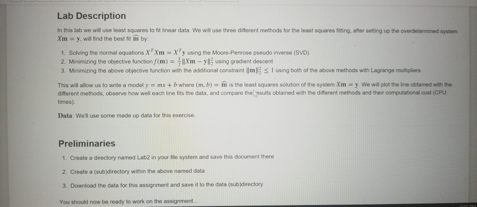
Lab Description In this lab we will use least squares to fit linear data. We will use three different methods for the least squares fitting, after setting up the overdetermined system Xm - y, will ind the best fit m by: 1. Solving the normal equations XTXm XTy using the Moore-Penrose pseudo inverse (SVD) 2. Minimizing the objective function/(m) = 1Xm-yl. using gradient descent 3. Minimizing the above objective function with the additional constraint lImll S 1 using both of the above methods with Lagrange multipliers This will allow us to write a model y mr + b where (m. b) = m is the least squares solution of the system Xm-y. We will plot the line obtained with the different methods, observe how well each line fits the data, and compare the esults obtained with the different methods and their computational cost (CPu times). Data: We'll use some made up data for this exercise. Preliminaries 1. Create a directory named Lab2 in your file system and save this document there 2. Create a (sub)directory within the above named data 3. Download the data for this assignment and save it to the data (sub)directory You should now be ready to work on the assignment Lab Description In this lab we will use least squares to fit linear data. We will use three different methods for the least squares fitting, after setting up the overdetermined system Xm - y, will ind the best fit m by: 1. Solving the normal equations XTXm XTy using the Moore-Penrose pseudo inverse (SVD) 2. Minimizing the objective function/(m) = 1Xm-yl. using gradient descent 3. Minimizing the above objective function with the additional constraint lImll S 1 using both of the above methods with Lagrange multipliers This will allow us to write a model y mr + b where (m. b) = m is the least squares solution of the system Xm-y. We will plot the line obtained with the different methods, observe how well each line fits the data, and compare the esults obtained with the different methods and their computational cost (CPu times). Data: We'll use some made up data for this exercise. Preliminaries 1. Create a directory named Lab2 in your file system and save this document there 2. Create a (sub)directory within the above named data 3. Download the data for this assignment and save it to the data (sub)directory You should now be ready to work on the assignment