Lesson: Extreme Value Theorem, Mean Value Theorem, First Derivative Test, Concavity and

Points of Inflection (i.e. second derivative test), Limits at Infinity and Curve Sketching

General Instructions: Consider the given steps to sketch the graph of the functions.

Functions to be graphed:

5.) y= 1-3x+5x²-x³

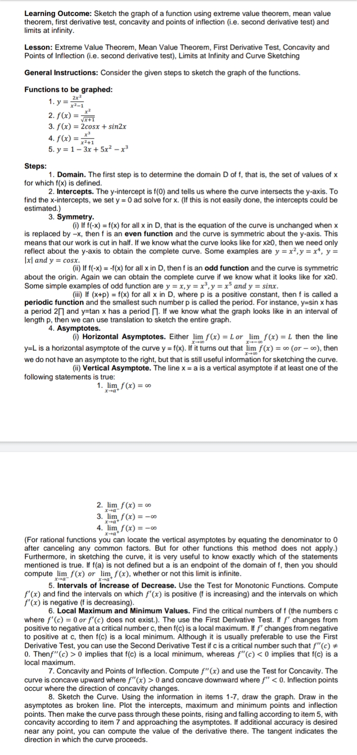
Learning Outcome: Sketch the graph of a function using extreme value theorem, mean value theorem, first derivative test, concavity and points of inflection (i.e. second derivative test) and limits at infinity. Lesson: Extreme Value Theorem, Mean Value Theorem, First Derivative Test, Concavity and Points of Inflection (i.e. second derivative test), Limits at Infinity and Curve Sketching General Instructions: Consider the given steps to sketch the graph of the functions. Functions to be graphed: 1. y = 2x2 72-1 2. f (x) = 3. f(x) = 2cosx + sin2x 4. f (x)= 5. y = 1 - 3x + 5x2 - x3 Steps: for which f(x) is defined. 1. Domain. The first step is to determine the domain D of f, that is, the set of values of x 2. Intercepts. The y-intercept is f(0) and tells us where the curve intersects the y-axis. To find the x-intercepts, we set y = 0 ad solve for x. (If this is not easily done, the intercepts could be estimated.) 3. Symmetry. (i) If f(-x) = f(x) for all x in D, that is the equation of the curve is unchanged when x is replaced by -x, then f is an even function and the curve is symmetric about the y-axis. This means that our work is cut in half. If we know what the curve looks like for x20, then we need only reflect about the y-axis to obtain the complete curve. Some examples are y = x, y = x*, y = Ixl and y = cosx. (ii) If f(-x) = -f(x) for all x in D, then f is an odd function and the curve is symmetric about the origin. Again we can obtain the complete curve if we know what it looks like for x20. Some simple examples of odd function are y = x, y = x , y = x and y = sinx. (i) If (x+p) = f(x) for all x in D, where p is a positive constant, then f is called a periodic function and the smallest such number p is called the period. For instance, y=sin x has a period 2/ and y=tan x has a period . If we know what the graph looks like in an interval of length p, then we can use translation to sketch the entire graph. 4. Asymptotes. (i) Horizontal Asymptotes. Either lim f(x) = Lor lim f(x) = L then the line X-4 -00 y=L is a horizontal asymptote of the curve y = f(x). If it turns out that lim f(x) = co (or - co), then X-+00 we do not have an asymptote to the right, but that is still useful information for sketching the curve. (ii) Vertical Asymptote. The line x = a is a vertical asymptote if at least one of the following statements is true: 1. lim f(x) = 00 x -at 2. lim f (x) = 00 3. lim f (x) = -co x-at 4. lim f (x) = -co x-at (For rational functions you can locate the vertical asymptotes by equating the denominator to 0 after canceling any common factors. But for other functions this method does not apply.) Furthermore, in sketching the curve, it is very useful to know exactly which of the statements mentioned is true. If f(a) is not defined but a is an endpoint of the domain of f, then you should compute lim f(x) or lim, f(x), whether or not this limit is infinite. x-at 5. Intervals of Increase of Decrease. Use the Test for Monotonic Functions. Compute f'(x) and find the intervals on which f'(x) is positive (f is increasing) and the intervals on which f'(x) is negative (f is decreasing). 6. Local Maximum and Minimum Values. Find the critical numbers of f (the numbers c where f'(c) = 0 or f'(c) does not exist.). The use the First Derivative Test. If f' changes from positive to negative at a critical number c, then f(c) is a local maximum. If f' changes from negative to positive at c, then f(c) is a local minimum. Although it is usually preferable to use the First Derivative Test, you can use the Second Derivative Test if c is a critical number such that f"(c) # 0. Thenf"(c) > 0 implies that f(c) is a local minimum, whereas f"(c) 0 and concave downward where f"